🧠 关键要点
⚙️ 环境设置
安装 conda:
在创建环境之前,请确保 conda 已安装在你的系统中。
保存 yml 内容:
将 yml 选项卡中的内容保存为文件
environment.yml。
创建环境:
打开终端或命令提示符。
运行以下命令:
conda env create -f environment.yml
激活环境:
创建好环境后,使用以下命令激活它:
conda activate <environment_name>请将
<environment_name>替换为environment.yml文件中指定的环境名称。该名称在 yml 文件中如下所示:name: <environment_name>
验证安装:
通过运行以下命令,检查环境是否创建成功:
conda env list
name: paired-integration
channels:
  - conda-forge
  - bioconda
  - defaults
dependencies:
  - conda-forge::python=3.12
  - conda-forge::scanpy=1.11.5
  - conda-forge::r-base=4.4
  - conda-forge::r-seurat=5.1
  - bioconda::bioconductor-singlecellexperiment
  - conda-forge::rpy2=3.6
  - bioconda::anndata2ri=1.3
  - conda-forge::pytorch-cpu
  - conda-forge::pip
  - pip:
      - muon==0.1.7
      - pysam
      - mofapy2==0.7.2
      - scib==1.1.6
      - scvi-tools==1.4.1
研究动机
多种单细胞技术已能在同一个细胞中测量不同模态(modality),即不同类型的生物学信息。例如,转录组与表位联合测序(Cellular Indexing of Transcriptomes and Epitopes by Sequencing, CITE-seq)同时测量基因表达和表面蛋白丰度;10x Multiome 测定(Assay)则配对获取 RNA 测序(RNA Sequencing, RNA-seq)和转座酶可及染色质测序(assay for transposase-accessible chromatin with high-throughput sequencing, ATAC-seq)数据,联合描述基因表达与染色质可及性(chromatin accessibility)。
整合多模态数据的目标,是利用互补信息构建更全面的细胞表示。不同模态的特征(feature)维度差异很大:RNA 数据矩阵可包含约 2 万至 3 万个基因,这不表示每个细胞都检出这么多基因;原教程中的蛋白面板从几个到约 200 个蛋白不等,而 ATAC 数据可包含超过 20 万个峰。这些是示例规模,不是技术的固定上限。各模态的数据分布也不同:RNA 计数(Count)常用负二项分布(Negative Binomial Distribution, NB)建模;ATAC 信号可按是否检出二值化,以伯努利分布(Bernoulli distribution)建模 Ashuach et al., 2021。原始 ATAC Count 也可采用泊松分布(Poisson distribution)建模 Martens et al., 2022。
本章演示多组学因子分析(Multi-Omics Factor Analysis, MOFA+)Argelaguet et al., 2020、加权最近邻(Weighted Nearest Neighbor, WNN)Hao et al., 2021、totalVI(Total Variational Inference)Gayoso et al., 2021 和 MultiVI Ashuach et al., 2021。示例使用 2021 年 NeurIPS 单细胞数据整合挑战中的 10x Multiome 和 CITE-seq 数据 Luecken et al., 2021。完整数据来自 12 位健康供体的骨髓单个核细胞(bone marrow mononuclear cell, BMMC),在四个实验地点测量,形成嵌套的批次效应(batch effect)。本章选择其中一个地点的三个批次演示整合。
选择整合方法需要结合任务与数据。这里使用单细胞整合基准评估(Single-Cell Integration Benchmarking, scIB)工具包 Luecken et al., 2022 定量比较整合结果。scIB 最初面向单模态的跨批次整合,因此这些分数只能反映多模态整合的部分性质,不能单独评判所有模态的信息是否都得到保留。原教程也指出,需要专门面向多模态任务的评估指标。
环境设置
import logging

import anndata as ad
import anndata2ri
import matplotlib.pyplot as plt
import muon as mu
import pandas as pd
import rpy2.rinterface_lib.callbacks
import scanpy as sc
import scib
import scipy
import scipy.io
import scvi
import seaborn as sns
from rpy2.robjects import pandas2ri

rpy2.rinterface_lib.callbacks.logger.setLevel(logging.ERROR)

pandas2ri.activate()
anndata2ri.activate()

%load_ext rpy2.ipython

import warnings

warnings.filterwarnings("ignore")
输出
During startup - Warning message:
Setting LC_CTYPE failed, using "C"
Global seed set to 0
/lustre/groups/ml01/workspace/anastasia.litinetskaya/miniconda3/envs/paired_integration_chapter/lib/python3.9/site-packages/pytorch_lightning/utilities/warnings.py:53: LightningDeprecationWarning: pytorch_lightning.utilities.warnings.rank_zero_deprecation has been deprecated in v1.6 and will be removed in v1.8. Use the equivalent function from the pytorch_lightning.utilities.rank_zero module instead.
  new_rank_zero_deprecation(
/lustre/groups/ml01/workspace/anastasia.litinetskaya/miniconda3/envs/paired_integration_chapter/lib/python3.9/site-packages/pytorch_lightning/utilities/warnings.py:58: LightningDeprecationWarning: The `pytorch_lightning.loggers.base.rank_zero_experiment` is deprecated in v1.7 and will be removed in v1.9. Please use `pytorch_lightning.loggers.logger.rank_zero_experiment` instead.
  return new_rank_zero_deprecation(*args, **kwargs)
/lustre/groups/ml01/workspace/anastasia.litinetskaya/miniconda3/envs/paired_integration_chapter/lib/python3.9/site-packages/rpy2/robjects/pandas2ri.py:351: DeprecationWarning: The global conversion available with activate() is deprecated and will be removed in the next major release. Use a local converter.
  warnings.warn('The global conversion available with activate() '
/lustre/groups/ml01/workspace/anastasia.litinetskaya/miniconda3/envs/paired_integration_chapter/lib/python3.9/site-packages/rpy2/robjects/numpy2ri.py:226: DeprecationWarning: The global conversion available with activate() is deprecated and will be removed in the next major release. Use a local converter.
  warnings.warn('The global conversion available with activate() '
/lustre/groups/ml01/workspace/anastasia.litinetskaya/miniconda3/envs/paired_integration_chapter/lib/python3.9/site-packages/rpy2/robjects/conversion.py:28: DeprecationWarning: The use of converter in module rpy2.robjects.conversion is deprecated. Use rpy2.robjects.conversion.get_conversion() instead of rpy2.robjects.conversion.converter.
  warnings.warn(
%%R
suppressPackageStartupMessages({
    library(Seurat)
})
set.seed(123)
    WARNING: The R package "reticulate" only fixed recently
    an issue that caused a segfault when used with rpy2:
    https://github.com/rstudio/reticulate/pull/1188
    Make sure that you use a version of that package that includes
    the fix.
CITE-seq 数据
先用 WNN、MOFA+ 和 totalVI 整合 CITE-seq 数据。该技术同时产生 RNA Count 和表面蛋白的抗体衍生标签(Antibody-Derived Tag, ADT)Count。具体原理见表面蛋白章节的 研究动机。下方读取的是原作者已预处理的文件,路径指向其共享文件系统;实际使用时需替换为自己的对应文件。不同模型将分别使用其中的归一化(normalization)数据或原始 Count 层。
数据准备
adt = sc.read(
    "/lustre/groups/ml01/workspace/anastasia.litinetskaya/data/neurips-cite/adt_pp.h5ad"
)
adt
AnnData object with n_obs × n_vars = 120502 × 136
obs: 'donor', 'batch', 'n_genes_by_counts', 'log1p_n_genes_by_counts', 'total_counts', 'log1p_total_counts', 'n_counts', 'outliers'
var: 'gene_ids', 'feature_types', 'n_cells_by_counts', 'mean_counts', 'log1p_mean_counts', 'pct_dropout_by_counts', 'total_counts', 'log1p_total_counts'
uns: 'batch_colors', 'donor_colors', 'neighbors', 'pca', 'umap'
obsm: 'X_isotypes', 'X_pca', 'X_pcahm', 'X_umap'
varm: 'PCs'
layers: 'counts'
obsp: 'connectivities', 'distances'rna = sc.read(
"/lustre/groups/ml01/workspace/anastasia.litinetskaya/data/neurips-cite/rna_hvg.h5ad"
)
rnaAnnData object with n_obs × n_vars = 90261 × 4000
obs: 'GEX_n_genes_by_counts', 'GEX_pct_counts_mt', 'GEX_size_factors', 'GEX_phase', 'ADT_n_antibodies_by_counts', 'ADT_total_counts', 'ADT_iso_count', 'cell_type', 'batch', 'ADT_pseudotime_order', 'GEX_pseudotime_order', 'Samplename', 'Site', 'DonorNumber', 'Modality', 'VendorLot', 'DonorID', 'DonorAge', 'DonorBMI', 'DonorBloodType', 'DonorRace', 'Ethnicity', 'DonorGender', 'QCMeds', 'DonorSmoker', 'is_train'
var: 'feature_types', 'gene_id', 'highly_variable', 'means', 'dispersions', 'dispersions_norm'
uns: 'dataset_id', 'genome', 'hvg', 'organism'
obsm: 'ADT_X_pca', 'ADT_X_umap', 'ADT_isotype_controls', 'GEX_X_pca', 'GEX_X_umap'
layers: 'counts'为缩短运行时间,仅保留 Site 1 的三个供体批次:s1d1、s1d2 和 s1d3。RNA 使用 batch 列,ADT 使用 donor 列筛选;应核对两列确实编码同一批次。
batches_to_keep = ["s1d1", "s1d2", "s1d3"]
rna = rna[rna.obs["batch"].isin(batches_to_keep)]
adt = adt[adt.obs["donor"].isin(batches_to_keep)]
这里只分析两种模态共有的细胞。先检查两个对象的 .obs_names,统一细胞条形码(cell barcode, CB)与批次后缀的格式,并确认名称唯一。随后用同一份共有名称列表索引两个对象,使细胞集合和行序一致。
adt.obs_namesIndex(['AAACCCAAGGATGGCT-1-0-0-0-0-0-0-0-0-0-0-0',
'AAACCCAAGGCCTAGA-1-0-0-0-0-0-0-0-0-0-0-0',
'AAACCCAAGTGAGTGC-1-0-0-0-0-0-0-0-0-0-0-0',
'AAACCCACAAGAGGCT-1-0-0-0-0-0-0-0-0-0-0-0',
'AAACCCACATCGTGGC-1-0-0-0-0-0-0-0-0-0-0-0',
'AAACCCACATTCTCTA-1-0-0-0-0-0-0-0-0-0-0-0',
'AAACCCAGTCCGCAGT-1-0-0-0-0-0-0-0-0-0-0-0',
'AAACCCAGTGCATACT-1-0-0-0-0-0-0-0-0-0-0-0',
'AAACCCAGTTGACGGA-1-0-0-0-0-0-0-0-0-0-0-0',
'AAACCCATCGATACTG-1-0-0-0-0-0-0-0-0-0-0-0',
...
'TTTGGTTCATGTTACG-1-1-0-0-0', 'TTTGGTTGTCTCACAA-1-1-0-0-0',
'TTTGGTTTCCCATTCG-1-1-0-0-0', 'TTTGGTTTCCGTCCTA-1-1-0-0-0',
'TTTGGTTTCTTGCGCT-1-1-0-0-0', 'TTTGTTGAGAGTCTGG-1-1-0-0-0',
'TTTGTTGCAGACAATA-1-1-0-0-0', 'TTTGTTGCATGTTACG-1-1-0-0-0',
'TTTGTTGGTAGTCACT-1-1-0-0-0', 'TTTGTTGTCGCGCTGA-1-1-0-0-0'],
dtype='object', length=24326)rna.obs_namesIndex(['GCATTAGCATAAGCGG-1-s1d1', 'TACAGGTGTTAGAGTA-1-s1d1',
'AGGATCTAGGTCTACT-1-s1d1', 'GTAGAAAGTGACACAG-1-s1d1',
'TCCGAAAAGGATCATA-1-s1d1', 'CTCCCAATCCATTGGA-1-s1d1',
'GACCAATCAATTTCGG-1-s1d1', 'TTCCGGTAGTTGTAAG-1-s1d1',
'ACCTGTCAGGACTGGT-1-s1d1', 'TTCGATTTCAGGACAG-1-s1d1',
...
'GTGGTTAGTCGAGTTT-1-s1d3', 'TGAGACTCAATAGTAG-1-s1d3',
'CATGAGTTCAGCAGAG-1-s1d3', 'GCTACAACAGTGCGCT-1-s1d3',
'AGAAATGAGTGCCTCG-1-s1d3', 'AACAAAGGTTGGTACT-1-s1d3',
'TGACAGTCATGGCTGC-1-s1d3', 'CTGGCAGGTCTCACGG-1-s1d3',
'GTAACCATCGGAGTGA-1-s1d3', 'GAGTTGTCAGTCGGAA-1-s1d3'],
dtype='object', length=16311)adt.obs_names = [
name.split("-")[0] + "-" + name.split("-")[1] + "-" + batch
for batch, name in zip(adt.obs["donor"], adt.obs_names, strict=False)
]common_idx = list(set(rna.obs_names).intersection(set(adt.obs_names)))
rna = rna[common_idx].copy()
adt = adt[common_idx].copy()给 adt 对象中的蛋白名称添加 PROT_ 前缀,避免与 RNA 基因名称重复;这只改变名称,不改变测量值。
adt.var_names = ["PROT_" + name for name in adt.var_names]创建 MuData 对象,将 RNA 和 ADT 两种模态分别保存在其中。
mdata = mu.MuData({"rna": rna, "adt": adt})
mdata把 RNA AnnData 中的 batch 和 cell_type 两列复制到 MuData 对象的 .obs 中,供后续可视化着色使用。
mdata.obs["batch"] = rna.obs["batch"].copy()
mdata.obs["cell_type"] = rna.obs["cell_type"].copy()加权最近邻(WNN)
WNN 根据各模态的低维表示学习细胞特异的模态权重,再据此寻找多模态邻居并构建联合图;权重并非全体细胞共用的一组常数。随后可用 WNN 图引导 RNA 表达的有监督主成分分析(Supervised Principal Component Analysis, sPCA),得到潜在空间(latent space)中的嵌入(Embedding),用于映射等后续任务。
先使用 anndata2ri 软件包(https://
adata_ = ad.AnnData(adt.X.copy())
adata_.obs_names = adt.obs_names.copy()
adata_.var_names = adt.var_names.copy()
adata_.obs["batch"] = adt.obs["donor"].copy()
adata_.obsm["harmony_pca"] = adt.obsm["X_pcahm"].copy()
%%R -i adata_
# indicate that data is stored in .X of AnnData object
adt = as.Seurat(adata_, data='X', counts=NULL)
# the assay is called "originalexp" by default, we rename it to "ADT"
adt <- RenameAssays(object = adt, originalexp = "ADT", verbose=FALSE)
adtAn object of class Seurat
136 features across 16294 samples within 1 assay
Active assay: ADT (136 features, 0 variable features)
1 dimensional reduction calculated: harmony_pca
对 RNA 数据执行同样的转换。
adata_ = ad.AnnData(rna.X.copy())
adata_.obs_names = rna.obs_names.copy()
adata_.var_names = rna.var_names.copy()
adata_.obs["cell_type"] = rna.obs["cell_type"].copy()
adata_.obs["batch"] = rna.obs["batch"].copy()
%%R -i adata_
rna = as.Seurat(adata_, data='X', counts=NULL)
rnaAn object of class Seurat
4000 features across 16294 samples within 1 assay
Active assay: originalexp (4000 features, 0 variable features)
将两种 Assay 放入同一个 Seurat 对象,并把默认的 RNA Assay 名称改为 RNA。
%%R
cite <- rna
cite[["ADT"]] <- CreateAssayObject(data = adt@assays$ADT@data)
%%R
cite <- RenameAssays(object = cite, originalexp = "RNA", verbose=FALSE) 多批次数据需要评估批次效应。WNN 本身不负责批次校正(batch correction),可先分别校正每个模态,例如使用 Seurat 的 FindIntegrationAnchors() 和 IntegrateData()(参见 https://
%%R
# TODO need to change after we have the preprocessed data, for now RNA is not batch-corrected
DefaultAssay(cite) <- "RNA"
VariableFeatures(cite) <- rownames(cite)
cite <- ScaleData(cite, verbose=FALSE)
cite <- RunPCA(cite, verbose=FALSE)
%%R
cite@reductions$harmony_pca <- adt@reductions$harmony_pca
citeAn object of class Seurat
4136 features across 16294 samples within 2 assays
Active assay: RNA (4000 features, 4000 variable features)
1 other assay present: ADT
2 dimensional reductions calculated: pca, harmony_pca
按照 WNN 教程,将各模态的降维(dimensionality reduction)结果传给 FindMultiModalNeighbors。本例使用 RNA 的前 50 个 PCA 维度与 ADT 的前 30 个 Harmony PCA 维度,学习模态权重并生成多模态邻居及相关图。
%%R
cite <- FindMultiModalNeighbors(
    cite,
    reduction.list = list("pca", "harmony_pca"),
    dims.list = list(1:50, 1:30),
    modality.weight.name = "RNA.weight",
    verbose = FALSE
)
为得到可用于后续映射的 Embedding,调用 RunSPCA(),以 RNA 表达为输入、以 wsnn 图引导 sPCA,使表示反映联合图中的细胞关系。下面还基于 weighted.nn 计算统一流形近似与投影(Uniform Manifold Approximation and Projection, UMAP),并保存其模型。后续 RNA 查询数据到该多模态参考的映射见 高级多模态整合章节。
%%R
cite <- RunSPCA(cite, assay = "RNA", graph = "wsnn", npcs = 20)
cite <- RunUMAP(cite, nn.name = "weighted.nn", reduction.name = "wnn.umap", reduction.key = "wnnUMAP_", return.model=TRUE)
%%R
citeAn object of class Seurat
4136 features across 16294 samples within 2 assays
Active assay: RNA (4000 features, 4000 variable features)
1 other assay present: ADT
4 dimensional reductions calculated: pca, harmony_pca, spca, wnn.umap
将 Seurat 对象保存为 .rds 文件,供后续 高级多模态整合 章节使用。
%%R
saveRDS(cite, file = "wnn_ref.rds")
将 sPCA Embedding 传回 Python,存入 MuData 对象的 .obsm 中。
%%R -o spca
spca = Embeddings(object = cite[["spca"]])
mdata.obsm["X_spca"] = spca再提取 WNN 流程生成的 wknn 图。注意这里导出的是 wknn,而前面引导 sPCA 的是 wsnn;两者是不同的图表示。
%%R -o wnn
wnn <- as.data.frame(summary(cite@graphs$wknn))
稀疏图展开后的表格给出存在连接的细胞索引和边权。R 索引从 1 开始,Python 从 0 开始,因此把 i、j 两列各减 1;还需保证 Seurat 与 MuData 的细胞顺序一致。
wnn[:5]wnn["i"] = wnn["i"] - 1
wnn["j"] = wnn["j"] - 1
wnn[:5]将图重建为稀疏矩阵(sparse matrix),存入 MuData 对象的 .obsp 中。
mdata.obsp["wnn_connectivities"] = scipy.sparse.coo_matrix(
    (wnn["x"], (wnn["i"], wnn["j"]))
)
下面先调用 Scanpy 建立邻居结果所需的元数据,再用导入的 WNN 连接矩阵替换 connectivities,删除原 distances 后计算 UMAP。结果另存于 .obsm['X_umap_wnn']。也可以直接在 sPCA 表示上构建近邻图(nearest-neighbor graph)再计算 UMAP,但这与使用 WNN 图不是同一可视化输入。
# we won't actually need the neighbors
# but need to run this anyway as a little trick to make scanpy work with externally-computed neighbors
sc.pp.neighbors(mdata, use_rep="X_spca")
mdata.obsp["connectivities"] = mdata.obsp["wnn_connectivities"].copy()
# delete distances to make sure we are not using anything calculated with sc.pp.neighbors()
del mdata.obsp["distances"]
sc.tl.umap(mdata)
mdata.obsm["X_umap_wnn"] = mdata.obsm["X_umap"].copy()在 UMAP 上分别按细胞类型和批次着色。
mu.pl.embedding(
    mdata, color=["cell_type", "batch"], ncols=1, basis="umap_wnn", frameon=False
)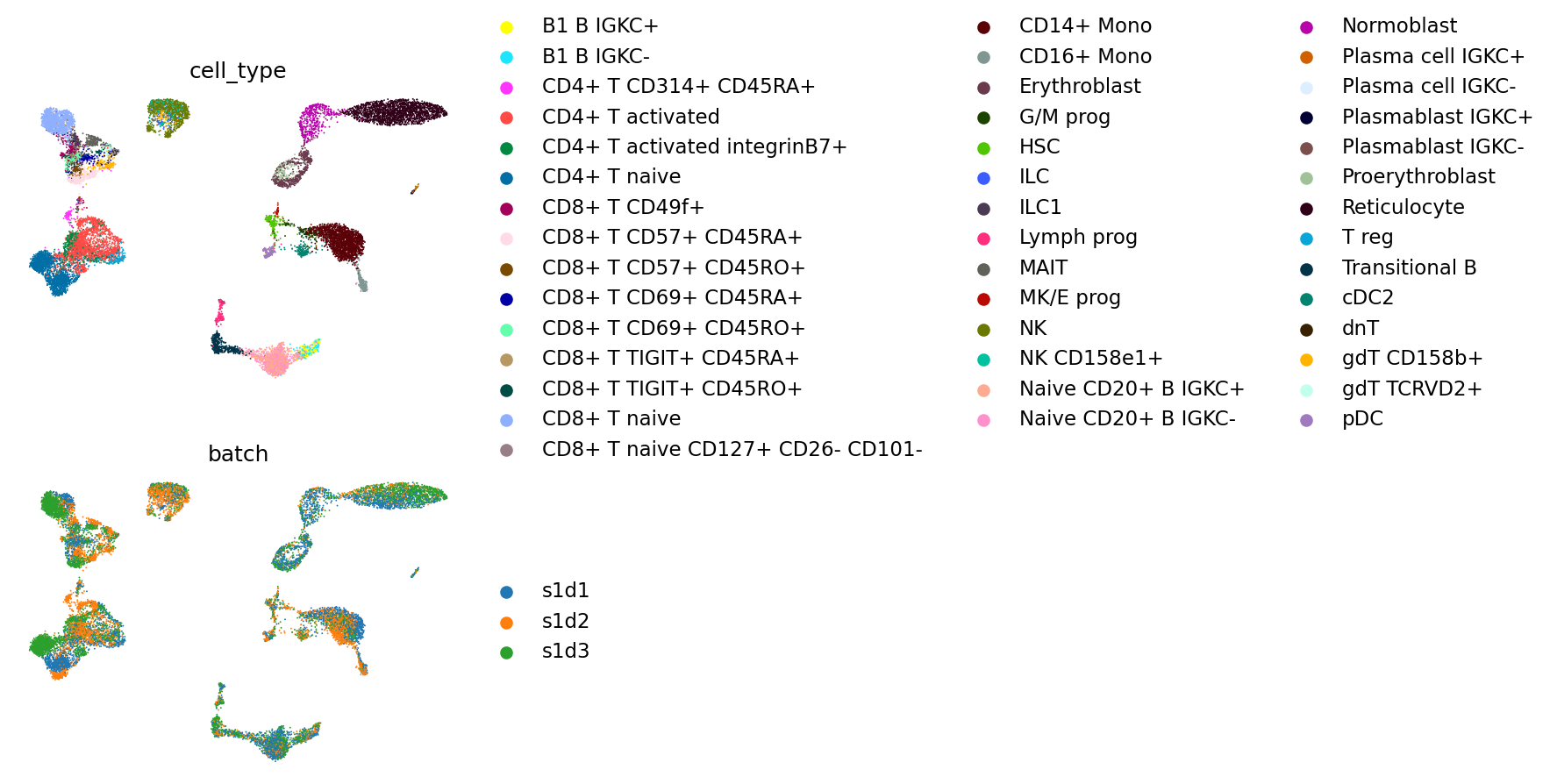
使用 sPCA Embedding 与 WNN 图计算以下 scIB 指标,定量比较整合结果。基于标签的指标依赖已有细胞类型注释,不能把已知标签的保留等同于保留了所有生物学差异。
生物学信息保留:
NMI_cluster/label、ARI_cluster/label、ASW_label和isolated_label_silhouette;批次校正:
ASW_label/batch、graph_conn。
scib_anndata = sc.AnnData(mdata.obsm["X_spca"]).copy()
scib_anndata.obs = mdata.obs.copy()
scib_anndata.obsp["connectivities"] = mdata.obsp["connectivities"].copy()
scib_anndata.obsm["X_spca"] = mdata.obsm["X_spca"].copy()
metrics_wnn = scib.metrics.metrics(
scib_anndata,
scib_anndata,
batch_key="batch",
label_key="cell_type",
embed="X_spca",
ari_=True,
nmi_=True,
silhouette_=True,
graph_conn_=True,
isolated_labels_asw_=True,
)
metrics_wnnNMI...
ARI...
Silhouette score...
Isolated labels ASW...
Graph connectivity...
即使整合前已对某个模态做过批次校正,仍应评估最终结果的批次混合情况。本例实际仅导入了 ADT 的 Harmony 校正表示,RNA 尚未按原文所称使用 scVI;解释这些分数时需保留这一差别。
多组学因子分析(MOFA+)
MOFA+ 是线性因子模型(linear factor model),用低秩因子矩阵与各模态的载荷(factor loading)矩阵描述输入数据的主要变异。因子值可作为低维 Embedding,用于可视化和其他分析;载荷则反映原始 feature 与各因子的关系。因子可帮助解释变异来源,但不保证每个因子都对应单一生物学过程。
MOFA+ 默认读取各模态的 .X。这里应提供按模态适当归一化的数据,并核对使用的似然。本例通过 groups_label 把 batch 指定为分组标签,进行多组建模;muon 的默认设置还会在组内中心化。它不是简单加入一个批次协变量(covariate)就自动消除全部批次效应,仍需检查因子中的批次与生物学结构。
下方设置 gpu_mode=True。如需在 GPU 上运行 MOFA+,还必须安装 CuPy(https://cupy.dev)并确保其与本机 CUDA 兼容;没有相应 GPU 环境时应使用 CPU 设置。
mu.tl.mofa(mdata, groups_label="batch", gpu_mode=True)输出
#########################################################
### __ __ ____ ______ ###
### | \/ |/ __ \| ____/\ _ ###
### | \ / | | | | |__ / \ _| |_ ###
### | |\/| | | | | __/ /\ \_ _| ###
### | | | | |__| | | / ____ \|_| ###
### |_| |_|\____/|_|/_/ \_\ ###
### ###
#########################################################
Loaded view='rna' group='s1d1' with N=5219 samples and D=4000 features...
Loaded view='rna' group='s1d3' with N=4975 samples and D=4000 features...
Loaded view='rna' group='s1d2' with N=6100 samples and D=4000 features...
Loaded view='adt' group='s1d1' with N=5219 samples and D=136 features...
Loaded view='adt' group='s1d3' with N=4975 samples and D=136 features...
Loaded view='adt' group='s1d2' with N=6100 samples and D=136 features...
Model options:
- Automatic Relevance Determination prior on the factors: True
- Automatic Relevance Determination prior on the weights: True
- Spike-and-slab prior on the factors: False
- Spike-and-slab prior on the weights: True
Likelihoods:
- View 0 (rna): gaussian
- View 1 (adt): gaussian
GPU mode is activated
######################################
## Training the model with seed 1 ##
######################################
Converged!
#######################
## Training finished ##
#######################
Saving model in /tmp/mofa_20230103-162506.hdf5...
Saved MOFA embeddings in .obsm['X_mofa'] slot and their loadings in .varm['LFs'].
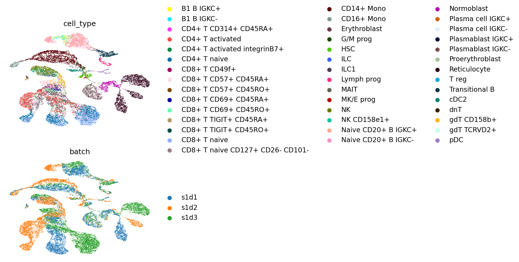
使用 X_mofa 表示计算邻居图和 UMAP,并把 UMAP 坐标存入 .obsm['X_umap_mofa']。
sc.pp.neighbors(mdata, use_rep="X_mofa")
sc.tl.umap(mdata)
mdata.obsm["X_umap_mofa"] = mdata.obsm["X_umap"].copy()再次按细胞类型和批次显示 UMAP。
mu.pl.embedding(
mdata, color=["cell_type", "batch"], ncols=1, basis="umap_mofa", frameon=False
)
计算与 WNN 相同的一组 scIB 指标。
scib_anndata = sc.AnnData(mdata.obsm["X_mofa"]).copy()
scib_anndata.obs = mdata.obs.copy()
scib_anndata.obsp["connectivities"] = mdata.obsp["connectivities"].copy()
scib_anndata.obsm["X_mofa"] = mdata.obsm["X_mofa"].copy()metrics_mofa = scib.metrics.metrics(
scib_anndata,
scib_anndata,
batch_key="batch",
label_key="cell_type",
embed="X_mofa",
ari_=True,
nmi_=True,
silhouette_=True,
graph_conn_=True,
isolated_labels_asw_=True,
)
metrics_mofaNMI...
ARI...
Silhouette score...
Isolated labels ASW...
Graph connectivity...
totalVI
totalVI 通过变分推断(variational inference, VI)联合建模配对的 RNA 和蛋白数据,将批次与蛋白背景纳入模型,以减少技术因素对联合潜在表示的影响。RNA 原始 Count 使用 NB 分布,蛋白原始 Count 使用前景与背景的 NB 混合分布;因此输入应是两种模态的原始 Count。模型旨在分离这些因素,但效果仍需用数据评估。下方先复制 RNA 对象,再将对应细胞的蛋白原始 Count 放入 protein_expression。
adata = mdata["rna"].copy()
adata.obsm["protein_expression"] = mdata["adt"].layers["counts"].A.copy()在 setup_anndata 中指定 RNA 原始 Count 位于 counts 层,并通过 batch_key="batch" 指定批次标签;蛋白原始 Count 的存储位置也要一并注册。
scvi.model.TOTALVI.setup_anndata(
adata,
protein_expression_obsm_key="protein_expression",
layer="counts",
batch_key="batch",
)No GPU/TPU found, falling back to CPU. (Set TF_CPP_MIN_LOG_LEVEL=0 and rerun for more info.)
INFO Generating sequential column names
初始化 totalVI 模型。
vae = scvi.model.TOTALVI(adata)INFO Computing empirical prior initialization for protein background.
使用默认训练参数拟合模型。
vae.train()输出
GPU available: True (cuda), used: True
TPU available: False, using: 0 TPU cores
IPU available: False, using: 0 IPUs
HPU available: False, using: 0 HPUs
LOCAL_RANK: 0 - CUDA_VISIBLE_DEVICES: [0]
Epoch 340/400: 85%|████████▌ | 340/400 [08:00<01:22, 1.37s/it, loss=1.65e+03, v_num=1]Epoch 00340: reducing learning rate of group 0 to 2.4000e-03.
Epoch 400/400: 100%|██████████| 400/400 [09:22<00:00, 1.37s/it, loss=1.64e+03, v_num=1]`Trainer.fit` stopped: `max_epochs=400` reached.
Epoch 400/400: 100%|██████████| 400/400 [09:22<00:00, 1.41s/it, loss=1.64e+03, v_num=1]
取得联合潜在表示,存入 .obsm['X_totalVI'],再基于该表示构建邻居图和 UMAP。赋值前应确认细胞顺序与 MuData 一致。
mdata.obsm["X_totalVI"] = vae.get_latent_representation()sc.pp.neighbors(mdata, use_rep="X_totalVI")
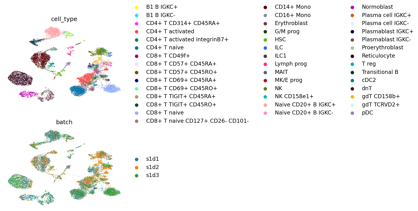
sc.tl.umap(mdata)mdata.obsm["X_umap_totalVI"] = mdata.obsm["X_umap"].copy()按细胞类型和批次显示 totalVI 的 UMAP。
mu.pl.embedding(
mdata, color=["cell_type", "batch"], ncols=1, basis="umap_totalVI", frameon=False
)
计算相同的 scIB 指标。
scib_anndata = sc.AnnData(mdata.obsm["X_totalVI"]).copy()
scib_anndata.obs = mdata.obs.copy()
scib_anndata.obsp["connectivities"] = mdata.obsp["connectivities"].copy()
scib_anndata.obsm["X_totalVI"] = mdata.obsm["X_totalVI"].copy()metrics_totalvi = scib.metrics.metrics(
scib_anndata,
scib_anndata,
batch_key="batch",
label_key="cell_type",
embed="X_totalVI",
ari_=True,
nmi_=True,
silhouette_=True,
graph_conn_=True,
isolated_labels_asw_=True,
)
metrics_totalvi输出
/lustre/groups/ml01/workspace/anastasia.litinetskaya/miniconda3/envs/paired_integration_chapter/lib/python3.9/site-packages/scib/metrics/metrics.py:293: DeprecationWarning: Call to deprecated function (or staticmethod) opt_louvain.
res_max, nmi_max, nmi_all = opt_louvain(
NMI...
ARI...
Silhouette score...
Isolated labels ASW...
Graph connectivity...
scIB 指标评估
合并各方法输出的 DataFrame,再计算总分并绘图。本例先分别对两项批次校正指标和四项生物学信息保留指标取平均,再按 scIB 的 0.4/0.6 权重组合,即 0.4 * batch_correction_metrics + 0.6 * bio_conservation_metrics。
metrics = pd.DataFrame([metrics_wnn[0], metrics_mofa[0], metrics_totalvi[0]])
metrics = metrics.set_index(pd.Index(["WNN", "MOFA+", "totalVI"]))
metrics = metrics.dropna(axis=1)
metricsmetrics["overall"] = (
0.4 * (metrics["ASW_label/batch"] + metrics["graph_conn"]) / 2
+ 0.6
* (
metrics["NMI_cluster/label"]
+ metrics["ARI_cluster/label"]
+ metrics["ASW_label"]
+ metrics["isolated_label_silhouette"]
)
/ 4
)
metricssns.scatterplot(data=metrics)
plt.legend(bbox_to_anchor=(1.05, 1), loc="upper left", borderaxespad=0)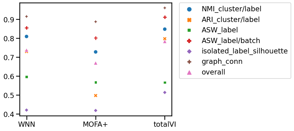
原教程报告 totalVI 在本例获得最高总分,并计划利用其 Embedding 结合 ADT 与 RNA 标记注释细胞群;本页后续实际转入 Multiome 示例,没有展开该注释流程。这个排序只对应当前数据、预处理和所选指标,尤其 WNN 的 RNA 输入尚未完成原文所称的批次校正,不能据此认定 totalVI 在所有任务中最优。方法选择应结合实验设计和具体下游目标。
Multiome 数据
下面用 MultiVI 整合配对的 RNA-seq 与 ATAC-seq 数据。WNN 和 MOFA+ 的总体框架也适用于这类数据,但需要改为合适的 ATAC 预处理、低维表示或似然设置,不能直接照搬 ADT 的处理。本节重点展示 MultiVI 的模型与输入准备。
数据准备
atac = sc.read(
    "/lustre/groups/ml01/workspace/anastasia.litinetskaya/data/neurips-multiome/atac_hvf.h5ad"
)
atac
AnnData object with n_obs × n_vars = 69249 × 40002
obs: 'GEX_pct_counts_mt', 'GEX_n_counts', 'GEX_n_genes', 'GEX_size_factors', 'GEX_phase', 'ATAC_nCount_peaks', 'ATAC_atac_fragments', 'ATAC_reads_in_peaks_frac', 'ATAC_blacklist_fraction', 'ATAC_nucleosome_signal', 'cell_type', 'batch', 'ATAC_pseudotime_order', 'GEX_pseudotime_order', 'Samplename', 'Site', 'DonorNumber', 'Modality', 'VendorLot', 'DonorID', 'DonorAge', 'DonorBMI', 'DonorBloodType', 'DonorRace', 'Ethnicity', 'DonorGender', 'QCMeds', 'DonorSmoker', 'cell_type_l2', 'cell_type_l1', 'cell_type_l3', 'assay'
var: 'feature_types', 'gene_id', 'n_cells', 'prop_shared_cells', 'variability_score'
uns: 'ATAC_gene_activity_var_names', 'dataset_id', 'genome', 'organism'
obsm: 'ATAC_gene_activity', 'ATAC_lsi_full', 'ATAC_lsi_red', 'ATAC_umap', 'GEX_X_pca', 'GEX_X_umap'
layers: 'binary', 'counts', 'cpm', 'tf-idf', 'tf-idf-binary', 'tf-idf-counts'rna = sc.read(
"/lustre/groups/ml01/workspace/anastasia.litinetskaya/data/neurips-multiome/rna_hvg.h5ad"
)
rnaAnnData object with n_obs × n_vars = 69249 × 4000
obs: 'GEX_pct_counts_mt', 'GEX_n_counts', 'GEX_n_genes', 'GEX_size_factors', 'GEX_phase', 'ATAC_nCount_peaks', 'ATAC_atac_fragments', 'ATAC_reads_in_peaks_frac', 'ATAC_blacklist_fraction', 'ATAC_nucleosome_signal', 'cell_type', 'batch', 'ATAC_pseudotime_order', 'GEX_pseudotime_order', 'Samplename', 'Site', 'DonorNumber', 'Modality', 'VendorLot', 'DonorID', 'DonorAge', 'DonorBMI', 'DonorBloodType', 'DonorRace', 'Ethnicity', 'DonorGender', 'QCMeds', 'DonorSmoker'
var: 'feature_types', 'gene_id', 'highly_variable', 'means', 'dispersions', 'dispersions_norm'
uns: 'ATAC_gene_activity_var_names', 'Site_colors', 'batch_colors', 'cell_type_colors', 'dataset_id', 'genome', 'hvg', 'organism'
obsm: 'ATAC_gene_activity', 'ATAC_lsi_full', 'ATAC_lsi_red', 'ATAC_umap', 'GEX_X_pca', 'GEX_X_umap', 'X_umap'
layers: 'counts'同样保留一个实验地点的三个批次,再创建 MuData。合并前需确认 RNA 与 ATAC 的细胞标识及对应关系。
batches_to_keep = ["s1d1", "s1d2", "s1d3"]
rna = rna[rna.obs["batch"].isin(batches_to_keep)]
atac = atac[atac.obs["batch"].isin(batches_to_keep)]
mdata_multiome = mu.MuData({"rna": rna, "atac": atac})
mdata_multiomemdata_multiome.obs["batch"] = mdata_multiome["rna"].obs["batch"].copy()
mdata_multiome.obs["cell_type"] = mdata_multiome["rna"].obs["cell_type"].copy()MultiVI
MultiVI 使用条件变分自编码器(Conditional Variational Autoencoder, CVAE)联合学习多模态表示。RNA 侧以原始 Count 建模;原文用 NB 概述,但本章环境指定的 scvi-tools 1.4.1 默认 gene_likelihood 为 zinb,即零膨胀负二项分布(Zero-Inflated Negative Binomial Distribution, ZINB),并非与 totalVI 的默认设置完全相同。ATAC 侧采用伯努利似然,拟合区域中是否检出信号。该版本在损失函数内以 x > 0 二值化目标,因此可输入原始 ATAC Count,不要求提前把整份输入改成二值。零值表示没有观测到信号,不能直接证明该区域在生物学上关闭。
n_genes = len(rna.var_names)
n_regions = len(atac.var_names)
这里采用 AnnData 接口,将基因与峰沿 feature 轴拼接:先分别转置,再用 ad.concat 拼接,最后转置回来。默认连接按共有细胞对齐;仍应核对细胞名称、基因在前峰在后的列顺序,以及两种模态的 counts 层。
adata_paired = ad.concat([rna.copy().T, atac.copy().T]).T
adata_paired.obs = adata_paired.obs.join(rna.obs[["cell_type", "batch"]])
adata_paired.obs["modality"] = "paired"
adata_paired
AnnData object with n_obs × n_vars = 17243 × 44002
obs: 'cell_type', 'batch', 'modality'
var: 'feature_types', 'gene_id'
layers: 'counts'adata_mvi = scvi.data.organize_multiome_anndatas(adata_paired)通过 layer='counts' 指定原始 Count 层;该参数传给 setup_anndata。这只选择输入数据位置,不会把归一化数值恢复为原始 Count。这里另以 modality 注册模态标签,并将实际 batch 作为分类协变量。
scvi.model.MULTIVI.setup_anndata(
    adata_mvi,
    batch_key="modality",
    categorical_covariate_keys=["batch"],
    layer="counts",
)
初始化 MultiVI,并指定基因数和区域数,使模型正确划分两类 feature。
mvi = scvi.model.MULTIVI(
    adata_mvi,
    n_genes=n_genes,
    n_regions=n_regions,
)
使用默认训练参数拟合 MultiVI。
mvi.train()输出
GPU available: True (cuda), used: True
TPU available: False, using: 0 TPU cores
IPU available: False, using: 0 IPUs
HPU available: False, using: 0 HPUs
/lustre/groups/ml01/workspace/anastasia.litinetskaya/miniconda3/envs/paired_integration_chapter/lib/python3.9/site-packages/pytorch_lightning/trainer/configuration_validator.py:267: LightningDeprecationWarning: The `Callback.on_epoch_end` hook was deprecated in v1.6 and will be removed in v1.8. Please use `Callback.on_<train/validation/test>_epoch_end` instead.
  rank_zero_deprecation(
LOCAL_RANK: 0 - CUDA_VISIBLE_DEVICES: [0]
Epoch 106/500:  21%|██        | 106/500 [11:30<42:46,  6.51s/it, loss=4.47e+03, v_num=1]
Monitored metric reconstruction_loss_validation did not improve in the last 50 records. Best score: 9223.312. Signaling Trainer to stop.
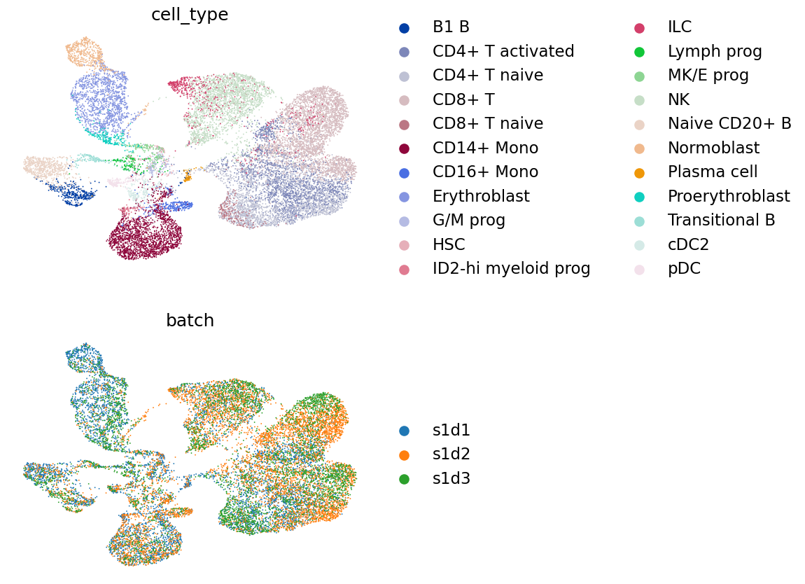
取得潜在 Embedding,在确认细胞顺序一致后写回 MuData,构建邻居图并计算 UMAP,分别查看细胞类型与批次。
mdata_multiome.obsm["X_multiVI"] = mvi.get_latent_representation()sc.pp.neighbors(mdata_multiome, use_rep="X_multiVI")
sc.tl.umap(mdata_multiome)mdata_multiome.obsm["X_umap_multiVI"] = mdata_multiome.obsm["X_umap"].copy()mu.pl.embedding(
mdata_multiome,
color=["cell_type", "batch"],
ncols=1,
basis="umap_multiVI",
frameon=False,
)
会话信息。
%%R
sessionInfo()
输出
R version 4.2.2 (2022-10-31)
Platform: x86_64-conda-linux-gnu (64-bit)
Running under: CentOS Linux 7 (Core)

Matrix products: default
BLAS/LAPACK: /lustre/groups/ml01/workspace/anastasia.litinetskaya/miniconda3/envs/paired_integration_chapter/lib/libopenblasp-r0.3.21.so

locale:
 [1] LC_CTYPE=C                 LC_NUMERIC=C
 [3] LC_TIME=en_US.UTF-8        LC_COLLATE=en_US.UTF-8
 [5] LC_MONETARY=en_US.UTF-8    LC_MESSAGES=en_US.UTF-8
 [7] LC_PAPER=en_US.UTF-8       LC_NAME=C
 [9] LC_ADDRESS=C               LC_TELEPHONE=C
[11] LC_MEASUREMENT=en_US.UTF-8 LC_IDENTIFICATION=C

attached base packages:
[1] stats4    tools     stats     graphics  grDevices utils     datasets
[8] methods   base

other attached packages:
 [1] Matrix_1.5-3                SingleCellExperiment_1.20.0
 [3] SummarizedExperiment_1.28.0 Biobase_2.58.0
 [5] GenomicRanges_1.50.0        GenomeInfoDb_1.34.1
 [7] IRanges_2.32.0              MatrixGenerics_1.10.0
 [9] matrixStats_0.63.0          S4Vectors_0.36.0
[11] BiocGenerics_0.44.0         SeuratObject_4.1.3
[13] Seurat_4.3.0

loaded via a namespace (and not attached):
  [1] Rtsne_0.16             colorspace_2.0-3       deldir_1.0-6
  [4] ellipsis_0.3.2         ggridges_0.5.4         XVector_0.38.0
  [7] spatstat.data_3.0-0    leiden_0.4.3           listenv_0.9.0
 [10] ggrepel_0.9.2          fansi_1.0.3            codetools_0.2-18
 [13] splines_4.2.2          polyclip_1.10-4        jsonlite_1.8.4
 [16] ica_1.0-3              cluster_2.1.4          png_0.1-8
 [19] uwot_0.1.14            shiny_1.7.4            sctransform_0.3.5
 [22] spatstat.sparse_3.0-0  compiler_4.2.2         httr_1.4.4
 [25] fastmap_1.1.0          lazyeval_0.2.2         cli_3.5.0
 [28] later_1.3.0            htmltools_0.5.4        igraph_1.3.5
 [31] gtable_0.3.1           glue_1.6.2             GenomeInfoDbData_1.2.9
 [34] RANN_2.6.1             reshape2_1.4.4         dplyr_1.0.10
 [37] Rcpp_1.0.9             scattermore_0.8        vctrs_0.5.1
 [40] spatstat.explore_3.0-5 nlme_3.1-161           progressr_0.12.0
 [43] lmtest_0.9-40          spatstat.random_3.0-1  stringr_1.5.0
 [46] globals_0.16.2         mime_0.12              miniUI_0.1.1.1
 [49] lifecycle_1.0.3        irlba_2.3.5.1          goftest_1.2-3
 [52] future_1.30.0          MASS_7.3-58.1          zlibbioc_1.44.0
 [55] zoo_1.8-11             scales_1.2.1           promises_1.2.0.1
 [58] spatstat.utils_3.0-1   parallel_4.2.2         RColorBrewer_1.1-3
 [61] reticulate_1.26        pbapply_1.6-0          gridExtra_2.3
 [64] ggplot2_3.4.0          stringi_1.7.8          rlang_1.0.6
 [67] pkgconfig_2.0.3        bitops_1.0-7           lattice_0.20-45
 [70] ROCR_1.0-11            purrr_1.0.0            tensor_1.5
 [73] patchwork_1.1.2        htmlwidgets_1.6.0      cowplot_1.1.1
 [76] tidyselect_1.2.0       parallelly_1.33.0      RcppAnnoy_0.0.20
 [79] plyr_1.8.8             magrittr_2.0.3         R6_2.5.1
 [82] generics_0.1.3         DelayedArray_0.24.0    pillar_1.8.1
 [85] fitdistrplus_1.1-8     survival_3.4-0         abind_1.4-5
 [88] RCurl_1.98-1.9         sp_1.5-1               tibble_3.1.8
 [91] future.apply_1.10.0    KernSmooth_2.23-20     utf8_1.2.2
 [94] spatstat.geom_3.0-3    plotly_4.10.1          grid_4.2.2
 [97] data.table_1.14.6      digest_0.6.31          xtable_1.8-4
[100] tidyr_1.2.1            httpuv_1.6.7           munsell_0.5.0
[103] viridisLite_0.4.1
- Ashuach, T., Gabitto, M. I., Jordan, M. I., & Yosef, N. (2021). MultiVI: deep generative model for the integration of multi-modal data. bioRxiv. 10.1101/2021.08.20.457057
- Martens, L. D., Fischer, D. S., Theis, F. J., & Gagneur, J. (2022). Modeling fragment counts improves single-cell ATAC-seq analysis. bioRxiv. 10.1101/2022.05.04.490536
- Argelaguet, R., Arnol, D., Bredikhin, D., Deloro, Y., Velten, B., Marioni, J. C., & Stegle, O. (2020). MOFA+: a statistical framework for comprehensive integration of multi-modal single-cell data. Genome Biology, 21(1), 111. 10.1186/s13059-020-02015-1
- Hao, Y., Hao, S., Andersen-Nissen, E., Mauck, W. M., Zheng, S., Butler, A., Lee, M. J., Wilk, A. J., Darby, C., Zager, M., Hoffman, P., Stoeckius, M., Papalexi, E., Mimitou, E. P., Jain, J., Srivastava, A., Stuart, T., Fleming, L. M., Yeung, B., … Satija, R. (2021). Integrated analysis of multimodal single-cell data. Cell, 184(13), 3573-3587.e29. https://doi.org/10.1016/j.cell.2021.04.048
- Gayoso, A., Steier, Z., Lopez, R., Regier, J., Nazor, K. L., Streets, A., & Yosef, N. (2021). Joint probabilistic modeling of single-cell multi-omic data with totalVI. Nature Methods, 18(3), 272–282. 10.1038/s41592-020-01050-x
- Luecken, M. D., Burkhardt, D. B., Cannoodt, R., Lance, C., Agrawal, A., Aliee, H., Chen, A. T., Deconinck, L., Detweiler, A. M., Granados, A. A., Huynh, S., Isacco, L., Kim, Y. J., Klein, D., KUMAR, B. D., Kuppasani, S., Lickert, H., McGeever, A., Mekonen, H., … Bloom, J. M. (2021). A sandbox for prediction and integration of DNA, RNA, and proteins in single cells. Thirty-Fifth Conference on Neural Information Processing Systems Datasets and Benchmarks Track (Round 2). https://openreview.net/forum?id=gN35BGa1Rt
- Luecken, M. D., Büttner, M., Chaichoompu, K., Danese, A., Interlandi, M., Mueller, M. F., Strobl, D. C., Zappia, L., Dugas, M., Colomé-Tatché, M., & Theis, F. J. (2022). Benchmarking atlas-level data integration in single-cell genomics. Nature Methods, 19(1), 41–50. 10.1038/s41592-021-01336-8