bulk 数据去卷积

本章介绍细胞类型去卷积（cell type deconvolution）的基本概念，涵盖输入数据的组织方式、预处理步骤及结果解读，并以 MuSiC 演示如何从 bulk 表达数据估计细胞类型组成。

背景¶

研究组织中细胞类型组成的差异，有助于理解疾病及其分子机制。首先，细胞类型之间的相互作用参与疾病进展和恢复。其次，组织整体的基因表达、蛋白质丰度等分子测量，往往随细胞类型组成而变化；只有了解这些组成，才能更好地区分细胞比例变化与细胞内部的分子变化。最后，识别疾病相关的细胞组成模式，还可能帮助确定治疗靶点，为临床研究提供线索。

细胞类型去卷积是一类计算方法，用于从异质组织的 bulk 分子数据推断各细胞群体的组成 Kuhn et al., 2012Schwartz, 2010Du et al., 2019Zaitsev et al., 2019。直接实验测量这些组成通常耗时且成本较高，去卷积因此为大规模研究提供了补充途径。许多方法采用线性回归（linear regression），其基本模型可写为：

$y = bX$

其中， $y$ 表示通过微阵列或 RNA 测序（RNA Sequencing, RNA-seq）等技术测得的 bulk 混合表达谱， $X$ 是细胞类型特征矩阵（signature matrix），每一行代表一种细胞类型的参考表达谱、每一列代表一个基因； $b$ 是待估计的混合权重行向量，通常希望用它表示各细胞类型的比例 Baron et al., 2016。不过，RNA 贡献比例不一定等于细胞数量比例：不同细胞类型的 RNA 含量可能不同，是否能估计细胞比例取决于方法的模型与校正。选择去卷积方法时，还需考虑参考数据是否缺少某些细胞类型、稀有类型的覆盖程度、归一化方式，以及用于拟合的特征（feature）（如标记基因（marker gene））的选择。

去卷积的效果在很大程度上取决于参考矩阵 $X$。其中汇集的表达信息反映了对组织内细胞异质性的已有认识，其覆盖范围和代表性影响细胞组成的估计 Aliee & Theis, 2021。早期参考谱常来自预先分选的细胞群体，例如先用荧光激活细胞分选（Fluorescence-Activated Cell Sorting, FACS）分离细胞，再测量表达。预设细胞类型和可用抗体会限制参考的覆盖范围。质谱流式细胞术（Cytometry by Time of Flight, CyTOF）也可刻画细胞组成，但并非用于后续 RNA 测量的活细胞分选技术 Monaco et al., 2019Aran et al., 2017。如今，单细胞 RNA 测序（Single-Cell RNA Sequencing, scRNA-seq）可为不同物种、组织和生物学条件建立参考谱，减少对预选细胞群体的依赖。不过，组织解离、捕获效率和抽样仍可能造成偏差，因此单细胞参考并不天然无偏 Aliee & Theis, 2021Newman et al., 2019。

方法¶

bulk 数据去卷积主要包括基于线性回归、基因集富集和非线性深度学习（deep learning, DL）的方法，以及其他建模思路。

线性回归是最常见的去卷积思路。这类方法直接拟合 $y = bX$ 所描述的混合关系，采用不同的正则化策略，通常利用较多基因作为 feature。

这类工具包括 CIBERSORTx Newman et al., 2019，MuSiC Wang et al., 2019，dtangle Hunt et al., 2018 和 DWLS Tsoucas et al., 2019。

基于富集的方法使用代表各细胞类型的基因集（gene set），分别计算其富集分数，再按具体方法进行校准或整合。这些分数可以提示细胞类型的相对富集程度，但通常不能直接解释为总和为 1 的细胞比例。细胞类型之间共享标记基因时，还可能出现交叉信号。xCell Aran et al., 2017 就是这类工具的一个例子，其主要输出是细胞类型富集分数。

非线性深度学习方法尝试学习更复杂的表达混合关系，在提高去卷积精度的同时保留生物学可解释性。这类方法的效果取决于训练数据与目标样本的匹配程度，尚不能笼统认定其优于其他方法。Scaden Menden et al., 2020 是其中一个例子。

已有多项研究对 bulk 数据去卷积方法开展基准测试，并得到一些相近的结论 Shen-Orr & Gaujoux, 2013Cobos et al., 2021Jin & Liu, 2021Nadel et al., 2021。在这些基准的测试条件下，使用 scRNA-seq 参考的方法表现较好，部分半监督方法的误差较高。参考中遗漏 bulk 混合物实际包含的细胞类型，通常会降低估计质量 Cobos et al., 2021。Cobos 等人建议：（1）输入使用线性尺度；（2）避免逐行缩放、逐列 最小–最大归一化（min–max normalization）、逐列 Z 分数标准化（z-score standardization）或分位数归一化（quantile normalization）；（3）优先考察 CIBERSORTx、FARDEEP 等表现较好的回归方法 Hao et al., 2019，若有 scRNA-seq 数据，可同时应用 DWLS、MuSiC 或 SCDC Dong et al., 2020 比较结果；（4）严格筛选标记基因，关注同一基因在表达量最高和次高的两种细胞类型之间的差异，以增强类型特异性；（5）参考矩阵应尽量包含混合物中的全部相关细胞类型 Cobos et al., 2021。归一化的影响尚无一致结论：Li 等人 Li et al., 2016 发现归一化策略对结果影响较大，但 Cobos 等人的基准未确认同样的结论。实际分析仍应遵循所用方法的输入要求，并结合目标数据验证 Cobos et al., 2021。

下面选择可在本地 R 环境中运行的 MuSiC 演示完整流程。CIBERSORTx 等工具也可作为比较方案；其使用方式和计算环境要求，应以工具当前提供的网页服务或容器文档为准。

MuSiC 的关键设计是利用多个单细胞参考样本，估计同一细胞类型在不同供体间的表达变异，从而对基因加权。应保留真实供体标签，并保证目标细胞类型在参考中有足够覆盖。若只有一个参考样本，就无法可靠估计供体间变异；若某些类型只在少数样本中出现，也可能使估计不稳定。应检查所用版本的输入要求和诊断结果，必要时选择适合现有参考的其他方法。

对 COVID-19 全血 bulk 样本进行去卷积¶

本例使用 MuSiC 分析 49 个全血 bulk RNA-seq 样本，其中 39 个来自 COVID-19 患者，10 个来自健康对照 Aschenbrenner et al., 2020；单细胞参考采用 COVID-19 患者的全血 scRNA-seq 数据 Schulte-Schrepping et al., 2020。

环境设置¶

加载数据¶

下方 data_file 是原作者的数据目录，复用时需先取得相应文件，并改为本机路径。首先读入单细胞和 bulk 数据，保留用于去卷积的数据在线性尺度上，不做 z-score 标准化或对数变换。部分基准表明，使用 scRNA-seq 参考时，线性尺度及适当的文库大小归一化（library-size normalization）有利于估计；具体仍需遵循方法要求 Jin & Liu, 2021Cobos et al., 2021。

数据预处理¶

读入数据后，先从单细胞参考中移除细胞类型 未明确 的记录。本例去除未注释、混合细胞和增殖细胞这三类标签，因为后两类可能跨越多种细胞类型。若其中包含 bulk 样本的重要成分，直接删除会使参考不完整；实际分析应尽量先细化注释。

注意：本例的单细胞数据已完成低质量细胞和基因的过滤，因此不再重复这部分质量控制（quality control, QC）。

去卷积方法对稀有细胞类型的比例估计通常更不稳定 Tsoucas et al., 2019。若决定去除参考中覆盖不足的类型，可设置最低细胞数阈值。原文将其记为 cellTypeNumCutOff，下方代码实际使用 rare_ct_cut_off = 50，并仅保留细胞数严格大于 50 的类型。阈值应依据数据选择；若删去的类型实际存在于 bulk 样本中，其信号可能被错误分配给其他类型。

在标记高变基因（Highly Variable Gene, HVG）之前，先取 bulk 数据与单细胞数据的基因交集，使两者使用相同的基因集合。

单细胞数据可视化¶

先将每个细胞的总 Count 归一化到 10,000，再标记 5,000 个 HVG。随后创建经过 log1p 变换的副本 adata_log，仅用于可视化；adata 仍保留线性尺度的归一化值。这里标记 HVG 并未将 adata 限制为这些基因。

接着用主成分分析（Principal Component Analysis, PCA）降维（dimensionality reduction），再用统一流形逼近与投影（Uniform Manifold Approximation and Projection, UMAP）展示细胞结构。

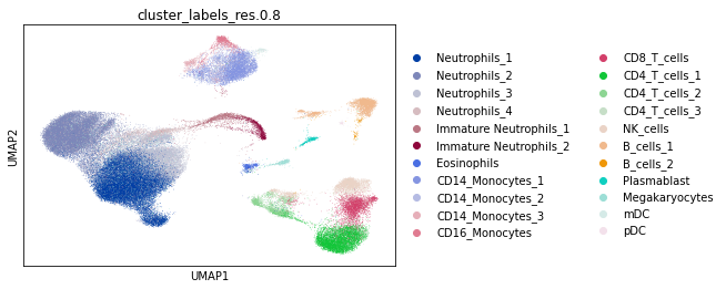
使用 MuSiC 进行去卷积¶

加载 R 接口¶

为调用 R 中的 MuSiC，需要把 Python 数据对象转换为 R 对象。若内存不足，可先进行子采样。下面的示例从每种细胞类型随机抽取至多 80 个细胞，没有按供体分层；实际使用时还需确保保留足够的供体和细胞类型覆盖。

若数据规模较小、无需子采样，可改用下面的完整 AnnData 副本。两种准备方式应择一使用；若顺序执行下面的代码，就会覆盖上一步的子采样结果。

运行 MuSiC¶

接下来准备传入 MuSiC 的数据：
1. adata_r：作为参考的单细胞表达矩阵。
2. cell_subsets_r：参考细胞的类型标签。
3. bulk：待去卷积的 bulk 样本表达矩阵。
4. sc_genes：参考矩阵的基因名。当前代码使用前面保留的全部共有基因，并未按 HVG 标记或独立标记基因列表进一步筛选。

MuSiC 分别为各 bulk 样本估计细胞比例，示例中的 9*** 表示样本名。需注意，下面的代码将全部参考细胞的 Sample 设为 1，没有保留真实供体，因此无法利用 MuSiC 所需的供体间表达变异；复用时应恢复供体标签，并按所用版本指定样本列和输入对象。传入的 adata_r 还沿用了逐细胞归一化值，这会改变细胞总 RNA 含量的信息，应核对所用 MuSiC 版本对参考 Count 和细胞大小校正的要求。此处保留原始示例，不能据此认定多供体分析已正确配置。

输出与验证¶

本例的比例估计整理为 N×M 矩阵，其中：
N（行数）：bulk 样本数。
M（列数）：参考中的细胞类型数。
每个元素表示一个样本中某种细胞类型的估计比例。以相对比例为输出的方法通常要求数值非负、每行之和为 1；富集分数等其他输出不满足这一解释，不能把所有去卷积工具的结果都视为细胞比例。

若有独立测得的细胞比例，可用于评估去卷积结果。本例用临床测得的中性粒细胞绝对数量，与各细胞类型的估计比例计算相关性。原示例观察到较高相关性，可作为一致性线索；但绝对数量与相对比例并非同一量，相关性高也不能证明比例估计已准确校准。

还可比较 COVID-19 患者与健康对照的估计细胞比例。下方代码对每种类型分别进行独立样本 Student t 检验（Student's t-test），沿用等方差假设，输出未经多重检验（multiple testing）校正的 p 值。该步骤仅作探索性演示；正式推断需评估分布与方差假设、多重检验、临床协变量，以及各比例总和为 1 带来的组成约束。

下面选取原始 p 值最小的细胞类型，用箱线图展示两组的估计比例分布。该图来自前面的数据筛选，不能作为独立验证。

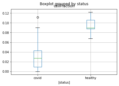
局限与常见陷阱¶

与预先分选的细胞群体相比，单细胞参考通常能覆盖更广的细胞类型，但仍可能遗漏难以捕获、稀有或特定状态的群体。参考缺失类型始终是去卷积的一项主要挑战 Cobos et al., 2021Jin & Liu, 2021。参考中细胞类型的数量和区分度也影响精度：若细分出的类型表达谱高度相似，模型更难可靠区分其贡献。不过，这不意味着可以任意删去 bulk 样本中实际存在的类型 Newman et al., 2019。

不少方法能较好估计主要细胞成分，但对稀有类型或表达谱高度相关的类型，表现差异较大。为缓解参考表达谱之间的共线性（collinearity），一些方法在去卷积前进行 feature 选择，筛出更能区分细胞类型的一组基因，形成特征基因列表（signature gene list）。这里减少的是所选基因空间中参考表达谱的相关性，并不改变细胞类型本身的生物学关系。

新方向¶

除上述方法外，还可使用以下工具改进 feature 选择，或解析细胞类型内部更细致的状态组成：

AutoGeneS Aliee & Theis, 2021 采用多目标 feature 选择，可整合进去卷积流程（pipeline）。它无需预先指定标记基因，而是同时降低不同细胞类型参考表达谱之间的相关性、增大它们之间的距离，从而选择区分度较高的基因。AutoGeneS 可用于单细胞实验或分选细胞群体等不同来源的参考谱。

CPM Frishberg et al., 2019 是一种细胞状态去卷积方法，以单细胞参考构建的状态空间为基础，识别每种细胞类型内部的组成变化。它更关注类型内部的变异，可用于发现特定亚群的相对丰度变化，或细胞沿连续轨迹分布的变化。

贡献者¶

我们衷心感谢以下人员的贡献：

作者¶

• Hananeh Aliee

• Amit Frishberg