🧠 关键要点
⚙️ 环境设置
安装 conda:
在创建环境之前,请确保 conda 已安装在你的系统中。
保存 yml 内容:
将 yml 选项卡中的内容保存为文件
environment.yml。
创建环境:
打开终端或命令提示符。
运行以下命令:
conda env create -f environment.yml
激活环境:
创建好环境后,使用以下命令激活它:
conda activate <environment_name>请将
<environment_name>替换为environment.yml文件中指定的环境名称。该名称在 yml 文件中如下所示:name: <environment_name>
验证安装:
通过运行以下命令,检查环境是否创建成功:
conda env list
name: gene-regulatory-networks-atac

channels:
  - conda-forge
  - anaconda
  - bioconda
dependencies:
  - conda-forge::python=3.8 # this package version is required for figR
  - conda-forge::r-base=4.2.2
  - conda-forge::r-umap
  - conda-forge::r-devtools
  - conda-forge::r-cairo
  - conda-forge::r-ggrastr
  - conda-forge::r-patchwork
  - conda-forge::r-gplots
  - conda-forge::r-networkd3 # network viz
  - conda-forge::r-r2d3 # network viz
  - conda-forge::r-webshot # network viz
  - conda-forge::phantomjs # network viz
  - conda-forge::r-imager # network viz
  - conda-forge::jupyterlab
  - conda-forge::jupyter_server=1.18.1
  - conda-forge::r-rmpfr
  - conda-forge::r-irkernel
  - conda-forge::r-dplyr
  - bioconda::bioconductor-zellkonverter>=1.8
  # - bioconda::bioconductor-bsgenome.hsapiens.ucsc.hg38=1.4.4 # this package will have to be installed while running
  - bioconda::bioconductor-complexheatmap
  - bioconda::bioconductor-motifmatchr
  - bioconda::bioconductor-rcistarget
  - bioconda::bioconductor-chromvar
研究动机
染色质可及性(chromatin accessibility)与基因表达之间具有机制上的联系:转录因子(Transcription Factor, TF)和其他表观遗传调节因子共同参与二者的调控。因此,联合分析这两类数据有助于理解基因调控 Spitz & Furlong, 2012。启动子(promoter)和近端或远端增强子(enhancer)参与表达调控,其可及性变化可作为活性变化的间接指标。在一定基因组距离内,例如小于 200 kbp,将转座酶可及染色质测序(Assay for Transposase-Accessible Chromatin with High-Throughput Sequencing, ATAC-seq)测得的可及性与 RNA 测序(RNA Sequencing, RNA-seq)测得的表达联系起来,可为基因调控网络(Gene Regulatory Network, GRN)提供候选边。以峰和基因为特征(feature)构建相关矩阵,可以筛选较强的峰–基因关联;这些相关性本身并不能证明直接调控或因果关系。
联合 RNA 与 ATAC feature 推断基因调控网络
本笔记本使用 FigR Kartha et al., 2022,以 NeurIPS 数据集中的一个供体为例演示 GRN 构建。准备阶段先调用 cisTopic Bravo González-Blas et al., 2019,从 ATAC 计数矩阵(Count matrix)中提取共同变化的可及性模式,即 主题(topic)。FigR 随后结合 TF 基序(motif)信息进行分析,并使用 chromVAR Schep et al., 2017 选择背景峰;具体的峰–基序匹配由 motifmatchr 完成。主要步骤改编自 FigR 针对 SHARE-seq 数据的 教程
撰写本章时,已有多种联合单细胞 RNA 和 ATAC 数据推断 GRN 的方法,但与前章类似,独立基准证据仍不足以确定哪种方法在大多数场景中最优。本章介绍的方法可作为探索性起点,得到的初步网络还需结合数据特点和独立证据验证。
安装并加载 FigR
# the installation of this package is required for the proper execution of this notebook.
if(!suppressMessages(require("FigR"))){
    suppressMessages(devtools::install_github("caleblareau/BuenColors")) # the package BuenColors is also a devtools dependency to install FigR.
    suppressMessages(devtools::install_github("buenrostrolab/FigR"))
}suppressMessages(library(FigR))使用 zellkonverter 将 h5ad 转换为 SingleCellExperiment
library(zellkonverter)
library(SingleCellExperiment)
先用 zellkonverter 读取完整的 NeurIPS 数据集,再根据 batch 列选择 s1d1 样本。本教程使用该样本的数据。注意,SingleCellExperiment 的行是 feature、列是细胞;下方上游示例把供体筛选向量放在行索引位置,实际复用时应按列筛选细胞。
sce <- readH5AD("../../data/openproblems_bmmc_multiome_genes_filtered.h5ad")
sce <- sce[colData(sce)$batch == 's1d1',]
为缩短计算时间,本例只选取部分 feature;RNA 子集保留所有已识别 TF,再抽取其他基因。
ncells = -1 # if using all cells
nfeatures_rna = 10000 # -1 if using all rna features
nfeatures_atac = 10000 # -1 if using all atac features
选出 s1d1 的细胞后,将 RNA 与 ATAC feature 分别存入两个对象。下方按行号拆分,依赖输入数据的 feature 排列;使用其他数据时应先核对 rownames(sce),再确定分界。
RNA <- sce[1:13431,]
ATAC <- sce[13432:nrow(sce),]
下载 hg38 的 TF 注释列表,并与仅使用 RNA 的教程保持一致的基因命名。也可使用 HumanTFs 等其他注释资源。
if(!file.exists('allTFs_hg38.txt'))
    download.file('https://raw.githubusercontent.com/aertslab/SCENICprotocol/master/example/allTFs_hg38.txt', 'allTFs_hg38.txt')
tf_names = rownames(read.table('allTFs_hg38.txt', row.names=1))
print(length(tf_names))
[1] 1797
# subset by cells:
if(ncells != -1){
    RNA <- RNA[,1:ncells]
    ATAC <- ATAC[,1:ncells]
}
if(nfeatures_rna != -1){

    # select all TFs and a subset of non-TFs
    is_tf <- rownames(RNA) %in% tf_names
    index_tf <- which(is_tf)
    index_not_tf <- which(!is_tf)
    set.seed(nfeatures_rna)
    RNA <- RNA[c(index_tf, sample(index_not_tf, nfeatures_rna - length(index_tf))),]
}
if(nfeatures_atac != -1){
    frac_atac <- rowSums(assay(ATAC)) / ncol(ATAC)
    acc_score <- abs(0.5 - frac_atac)
    peak_mask <- rownames(ATAC) %in% names(sort(acc_score))[1:nfeatures_atac]
    ATAC <- ATAC[peak_mask,]
}
print(c(dim(ATAC), dim(RNA)))
is_tf <- rownames(RNA) %in% tf_names
[1] 10000 6224 10000 6224
UMAP <- reducedDim(ATAC, 'GEX_X_umap')# counts variable (for later functions)
assay(ATAC) <- as(assay(ATAC), 'sparseMatrix')
counts(ATAC) <- assay(ATAC)还可按跨细胞表达情况预处理 RNA 对象;下面保留了去除全零基因的注释示例,当前不会执行。
# Remove genes with zero expression across all cells
# RNA <- RNA[Matrix::rowSums(RNA) != 0,]
准备并运行 cisTopic
cisTopic 使用潜在狄利克雷分配(Latent Dirichlet Allocation, LDA)学习主题,以概括 ATAC-seq 可及性数据中的共同变化。这里从单细胞转座酶可及染色质测序(single-cell assay for transposase-accessible chromatin using sequencing, scATAC-seq)数据建立 cisTopic 模型,将细胞的主题表示用于后续 FigR 分析。
如尚未安装 cisTopic,可通过 devtools 安装。作者环境中安装依赖约需十分钟,完成后可能需要重启内核。
if(!suppressMessages(require("cisTopic")))
suppressMessages(devtools::install_github("aertslab/cisTopic"))suppressMessages(library(cisTopic))指定可使用的 CPU 核心数(nCores),并根据实际计算资源调整。
nCores = 2cistopic_bkp_path <- "../../data/openproblems_bmmc_multiome_genes_filtered_atac_s1d1_counts_cisTopic.rds"
if(nfeatures_atac != -1)
cistopic_bkp_path <- paste0("../../data/openproblems_bmmc_multiome_genes_filtered_atac_s1d1_counts_cisTopic_npeaks", nfeatures_atac, ".rds")
print(c(file.exists(cistopic_bkp_path), cistopic_bkp_path))[1] "TRUE"
[2] "../../data/openproblems_bmmc_multiome_genes_filtered_atac_s1d1_counts_cisTopic_npeaks10000.rds"
拟合不同主题数的模型后,可结合两类曲线评估模型选择:
对数似然(log-likelihood)随主题数变化的曲线。如果逐渐进入平台,说明继续增加主题带来的拟合改善有限。
对数似然随主题数变化的增量或近似一阶导数。增量趋近于零、仅小幅波动时,提示额外主题带来的收益较小。
overwrite = TRUE # to visualize plots, this will always execute. Modify to FALSE to avoid replacing output from previous runs.
if(!file.exists(cistopic_bkp_path) || overwrite){
    # the number of topics to test
    n_topics = 1:25

    atac <- as.matrix(counts(ATAC))
    atac <- as.data.frame(atac)

    # we need to work out the names of the rownames, and replace - into : to match the chromosome:start-end required format by cisTopic
    chr <- sapply(strsplit(rownames(atac),"-"), `[`, 1)
    start <- sapply(strsplit(rownames(atac),"-"), `[`, 2)
    end <- sapply(strsplit(rownames(atac),"-"), `[`, 3)
    rownames(atac) <- paste0(chr, ':', start, '-', end)

    cisTopicObject <- createcisTopicObject(atac, project.name='neurips_s1d1')
    cisTopicObject <- runCGSModels(cisTopicObject, topic=c(n_topics), # , 5:15, 20, 25), # topic=c(2, 5:15, 20, 25),
                               seed=987, nCores=nCores, burnin = 90,
                               iterations = 100, addModels=FALSE)

    cisTopicObject <- selectModel(cisTopicObject, type='maximum')

    # cisTopicObject
    cisTopicObject <- runUmap(cisTopicObject, target='cell')

    topic.mat <- modelMatSelection(cisTopicObject, 'cell', 'Probability')
    topic.mat <- t(topic.mat)
    topic.mat <- as.matrix(topic.mat)
    saveRDS(topic.mat, cistopic_bkp_path)
}
[1] "Formatting data..."
[1] "Exporting data..."
[1] "Running models..."
Loading required package: umap
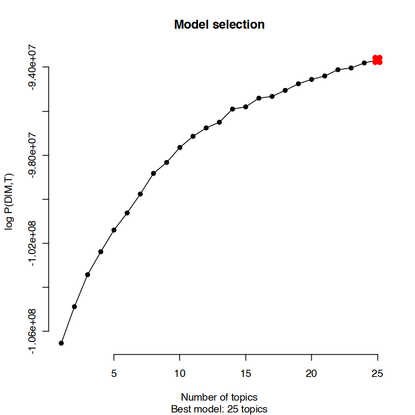
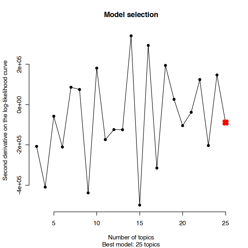
拟合并选择 cisTopic 模型后,读取已保存的细胞 × 主题概率矩阵。
cisAssign <- readRDS(cistopic_bkp_path)
dim(cisAssign) # Cells x Topics根据 cisTopic 的主题矩阵构建 k 近邻(k-Nearest Neighbors, kNN)关系;这里每个细胞取 30 个近邻。
library(dplyr)
library(FNN)
set.seed(123)
cellkNN <- get.knn(cisAssign, k = 30)$nn.index
dim(cellkNN)使用统一流形近似与投影(Uniform Manifold Approximation and Projection, UMAP)生成的嵌入(Embedding)展示细胞。下方绘图使用此前从 GEX_X_umap 读取的坐标,并非刚拟合的 cisTopic UMAP。
colData(ATAC)$cellAnnot <- colData(ATAC)$cell_typecolData(ATAC)$UMAP1 <- UMAP[,1]
colData(ATAC)$UMAP2 <- UMAP[,2]# Plot
library(ggplot2)
options(repr.plot.width=12, repr.plot.height=6)
colData(ATAC) %>% as.data.frame() %>% ggplot(aes(UMAP1,UMAP2,color=cellAnnot)) +
geom_point(size=0.5) + # scale_color_manual(values=annoCols)+
theme_classic() + guides(colour = guide_legend(override.aes = list(size=2))) + cowplot::theme_cowplot(font_family='Sans')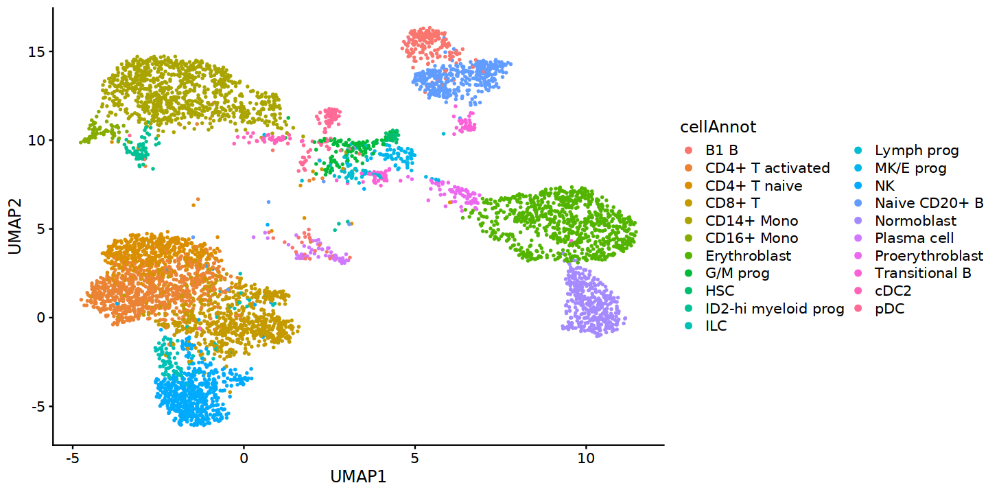
输入准备完成,接下来运行 FigR。
# if the hg38 genome is not installed successfully during environment building, it can be installed here.
# this might require a kernel restart
if(!suppressMessages(require('BSgenome.Hsapiens.UCSC.hg38'))){
    if (!require("BiocManager", quietly = TRUE))
        install.packages("BiocManager")
    BiocManager::install("BSgenome.Hsapiens.UCSC.hg38")
}suppressMessages(library(BSgenome.Hsapiens.UCSC.hg38))# check object dimensions
c(dim(ATAC), dim(RNA))指定可使用的 CPU 核心数(nCores),并根据实际计算资源调整。
为 runGenePeakcorr 准备 RNA 矩阵与带基因组坐标的 ATAC 对象;两者必须包含相同且顺序一致的细胞。
library(Matrix)
RNAmat <- as.matrix(assay(RNA))
dim(RNAmat)ATAC_df <- as.data.frame(as.matrix(counts(ATAC)))
# df <- as.data.frame(as.matrix(counts(ATAC)))ATAC_df$seqnames <- sapply(strsplit(rownames(ATAC_df),"-"), `[`, 1)
ATAC_df$start <- sapply(strsplit(rownames(ATAC_df),"-"), `[`, 2)
ATAC_df$end <- sapply(strsplit(rownames(ATAC_df),"-"), `[`, 3)ATAC_df <- subset(ATAC_df, grepl('chr', rownames(ATAC_df)))
dim(ATAC_df)ATAC.se <- makeSummarizedExperimentFromDataFrame(ATAC_df)
counts(ATAC.se) <- assay(ATAC.se)
assay(ATAC.se) <- as(assay(ATAC.se), 'sparseMatrix')使用两个 CPU 核心运行 FigR 的 runGenePeakcorr,计算峰–基因关联。
# This snippet can be run interactively, but it takes a long time.
nCores = 2
bkp_path_ciscorr <- '../../data/openproblems_bmmc_multiome_genes_filtered_s1d1_ciscorr.rds'
if(nfeatures_atac != -1)
    cistopic_bkp_path <- paste0("../../data/openproblems_bmmc_multiome_genes_filtered_s1d1_ciscorr_npeaks", nfeatures_atac, ".rds")

if(!file.exists(bkp_path_ciscorr)){
    cisCorr <- FigR::runGenePeakcorr(ATAC.se = ATAC.se,
                               RNAmat = RNAmat,
                               genome = "hg38", # One of hg19, mm10 or hg38
                               nCores = nCores,
                               p.cut = NULL, # Set this to NULL and we can filter later
                               n_bg = 250)
    saveRDS(cisCorr, bkp_path_ciscorr)
}
cisCorr <- readRDS(bkp_path_ciscorr)
按 p 值(p-value)筛选峰–基因关联。这里代码使用 pvalZ ≤ 0.05,并未进行多重检验(multiple testing)校正。
cisCorr.filt <- cisCorr %>% filter(pvalZ <= 0.05)
print(c('all associations', nrow(cisCorr)))
print(c('filtered associations', nrow(cisCorr.filt)))
[1] "all associations" "3914"
[1] "filtered associations" "674"
if(nrow(cisCorr.filt) == 0)
    print('increase the number of cells/peaks/genes to discover more associations')
stopifnot(nrow(cisCorr.filt) > 0)
计算峰–基因相关性后,FigR 将与同一基因显著相关的峰汇总为调控染色质域(Domain of Regulatory Chromatin, DORC),用聚合的可及性信号描述该基因附近的调控状态。随后结合 TF 表达与 DORC 可及性的相关性,以及相应峰中的 TF 基序富集,筛选候选调控关系。基序富集且相关性为正时,提示潜在激活作用;基序富集且相关性为负时,提示潜在抑制作用。这些仍是统计推断,不能直接证明 TF 结合或调控方向。
下图按显著关联峰的数量对基因排序,据此选择 DORC 基因;排序对象是所有候选基因,并不只限于 TF。
library(ggrepel)# Determine DORC genes
options(repr.plot.width=12, repr.plot.height=6)
cowplot_mono <- cowplot::theme_cowplot(font_family='sans')
dorcGenes <- cisCorr.filt %>% dorcJPlot(cutoff=2, # Default
returnGeneList = TRUE, family='sans') # + cowplot_mono
theme_set(theme_gray(base_family = "sans"))
dorcGenes + theme(font='roboto') # font problem during visualization of y/x axes (Roboto)NULL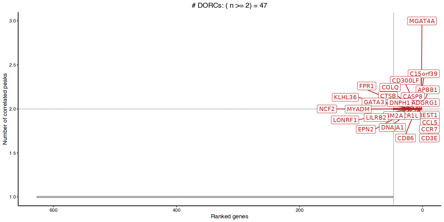
根据数据调整 DORC 峰数阈值,并检查是否有足够的 DORC 基因供后续分析。下方断言要求严格多于 30 个基因,与 runFigRGRN 默认的 DORC 近邻设置相对应。
stopifnot(length(dorcGenes) > 30)计算每个细胞的 DORC 可及性分数。
dorcMat <- getDORCScores(ATAC.se, dorcTab=cisCorr.filt, geneList=dorcGenes, nCores=nCores)
# Smooth DORC scores (using cell KNNs)
输出
Running DORC scoring for 47 genes: MGAT4A
ADGRG1
APBB1
BEST1
C15orf39
CASP8
CCL5
CCR7
CD300LF
CD3E
CD86
COLQ
CR1L
CTSB
DNAJA1
DNPH1
EPN2
FPR1
GATA3
GM2A
KLHL36
LILRB2
LONRF1
MYADM
NCF2
NFIA
NOLC1
P2RX1
PRF1
PRKCQ-AS1
PTCH1
RFPL1S
RHOQ
RXRA
SESN3
SLC16A6
SLC2A9
SMAD7
STRN3
SWAP70
TEC
THEMIS
TLE1
TM9SF2
TNRC6B
ZNF471
ZNRF1
........
Normalizing scATAC counts ..
SummarizedExperiment object input detected .. Centering counts under assayCentering counts for cells sequentially in groups of size  5000  ..

Computing centered counts for cells:  1  to  5000 ..
Computing centered counts per cell using mean reads in features ..

Computing centered counts for cells:  5001  to  6224 ..
Computing centered counts per cell using mean reads in features ..

Merging results..
Done!
Computing DORC scores ..
Running in parallel using  2 cores ..

Time Elapsed:  0.89201807975769 secs
stopifnot(nrow(cellkNN) == ncol(dorcMat))rownames(cellkNN) <- colnames(dorcMat)使用 smoothScoresNN 并行平滑分数前,加载 doParallel。细胞近邻矩阵与待平滑矩阵的细胞顺序必须一致,仅检查维度相同并不足够。
library(doParallel)# Smooth dorc scores using cell KNNs (k=30)
dorcMat.s <- smoothScoresNN(NNmat = cellkNN[,1:30], mat = dorcMat, nCores = nCores)Number of cells in supplied matrix: 6224
Number of genes in supplied matrix: 47
Number of nearest neighbors being used per cell for smoothing: 30
| | 0%Running in parallel using 2 cores ..
|======================================================================| 100%
Merging results ..
Time Elapsed: 14.4018683433533 secs
stopifnot(nrow(cellkNN) == ncol(RNAmat))rownames(cellkNN) <- colnames(RNAmat)# Smooth RNA using cell KNNs
# This takes longer since it's all genes
RNAmat.s <- smoothScoresNN(NNmat = cellkNN[,1:30], mat = RNAmat, nCores = nCores)Number of cells in supplied matrix: 6224
Number of genes in supplied matrix: 10000
Number of nearest neighbors being used per cell for smoothing: 30
| | 0%Running in parallel using 2 cores ..
|======================================================================| 100%
Merging results ..
Time Elapsed: 1.23741063674291 mins
library(ggplot2)
library(ggrastr)
# Visualize on pre-computed UMAP
umap.d <- as.data.frame(colData(ATAC)[,c("UMAP1","UMAP2")])DORC 分数计算后,可结合 TF 表达与候选靶基因关联,探索各细胞类型的调控特点。
print(length(dorcGenes))
print(dorcGenes)
[1] 47
[1] "MGAT4A" "ADGRG1" "APBB1" "BEST1" "C15orf39" "CASP8"
[7] "CCL5" "CCR7" "CD300LF" "CD3E" "CD86" "COLQ"
[13] "CR1L" "CTSB" "DNAJA1" "DNPH1" "EPN2" "FPR1"
[19] "GATA3" "GM2A" "KLHL36" "LILRB2" "LONRF1" "MYADM"
[25] "NCF2" "NFIA" "NOLC1" "P2RX1" "PRF1" "PRKCQ-AS1"
[31] "PTCH1" "RFPL1S" "RHOQ" "RXRA" "SESN3" "SLC16A6"
[37] "SLC2A9" "SMAD7" "STRN3" "SWAP70" "TEC" "THEMIS"
[43] "TLE1" "TM9SF2" "TNRC6B" "ZNF471" "ZNRF1"
下面以 核因子 I A(Nuclear Factor I A, NFIA) 为例,比较 NFIA 的 RNA 表达与该基因对应的 DORC 可及性。此处的 DORC 汇总与 NFIA 基因相关的峰,并不等同于所有含 NFIA 基序的峰。
marker_gene = 'NFIA'dorcg <- plotMarker2D(umap.d,dorcMat.s,markers = c(marker_gene),maxCutoff = "q0.99",
colorPalette = "brewer_heat") + ggtitle(paste0(marker_gene, ' DORC'))
Plotting NFIA
rnag <- plotMarker2D(umap.d,RNAmat.s,markers = c(marker_gene),maxCutoff = "q0.99",
                     colorPalette = "brewer_purple") + ggtitle(paste0(marker_gene, ' RNA'))
Plotting NFIA
使用 patchwork 并排展示 dorcg 与 rnag,在同一细胞坐标中比较 NFIA 的 DORC 分数和 RNA 表达。
options(repr.plot.width=12, repr.plot.height=6)
library(patchwork)
dorcg + cowplot_mono + rnag + cowplot_mono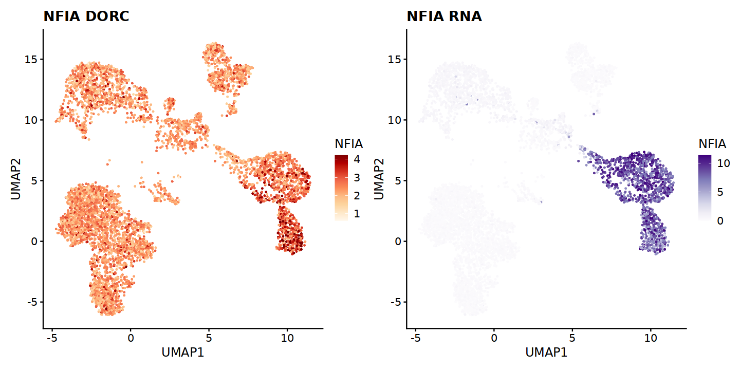
两幅图中的 NFIA 表达与 DORC 分数并不完全一致:有些细胞群体的 RNA 表达较高,对应的 DORC 信号却未同步升高。这说明两种测量提供不同层面的信息;不能仅凭该图判断 NFIA 蛋白是否结合了某些峰。
dim(dorcMat.s)figR.d <- runFigRGRN(ATAC.se = ATAC.se, # Must be the same input as used in runGenePeakcorr()
dorcTab = cisCorr.filt, # Filtered peak-gene associations
genome = "hg38",
dorcMat = dorcMat.s,
rnaMat = RNAmat.s,
nCores = nCores)输出
Assuming peak indices in Peak field

Removing genes with 0 expression across cells ..
Getting peak x motif matches ..
Determining background peaks ..
Using  50  iterations ..

Testing  626  TFs
Testing  47  DORCs
Running FigR using 2 cores ..
  |======================================================================| 100%Finished!
Merging results ..
结果可视化
下图展示 TF–DORC 调控评分。横轴 Corr.log10P 和纵轴 Enrichment.log10P 分别是相关性与基序富集检验的带符号 −log10(p),并非原始相关系数和富集倍数。颜色表示 FigR 的综合调控分数。右上方可提示候选激活因子,左上方可提示候选抑制因子;这些方向应作为待验证假设。
require(ggplot2)
require(ggrastr)
require(BuenColors) # https://github.com/caleblareau/BuenColors

options(repr.plot.width=10, repr.plot.height=8)

figR.d %>%
  ggplot(aes(Corr.log10P,Enrichment.log10P,color=Score)) +
  ggrastr::geom_point_rast(size=0.01,shape=16) +
  theme_classic() +
  scale_color_gradientn(colours = jdb_palette("solar_extra"),limits=c(-3,3),oob = scales::squish,breaks=scales::breaks_pretty(n=3)) +
  cowplot_mono + cowplot::theme_cowplot(font_family='sans' )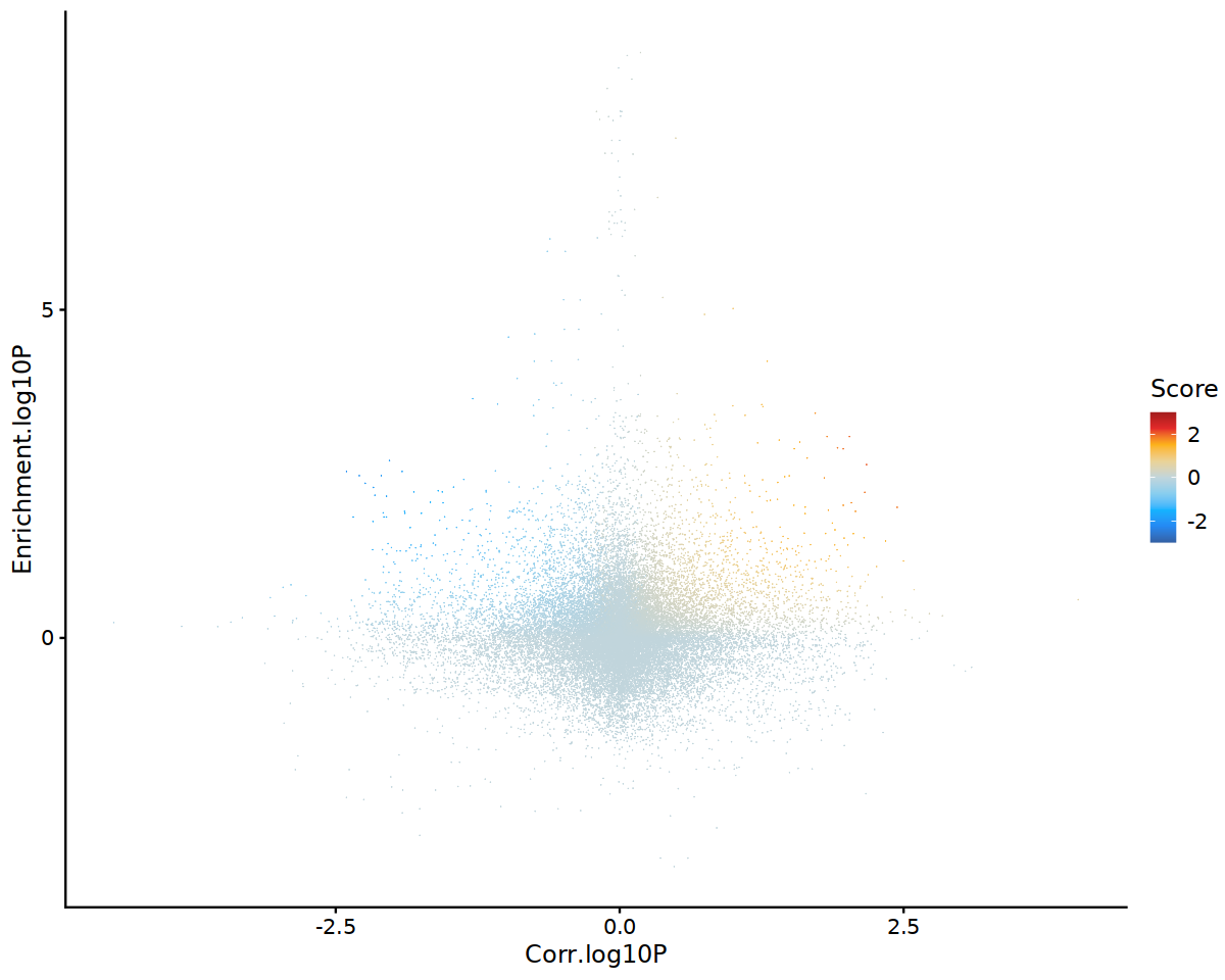
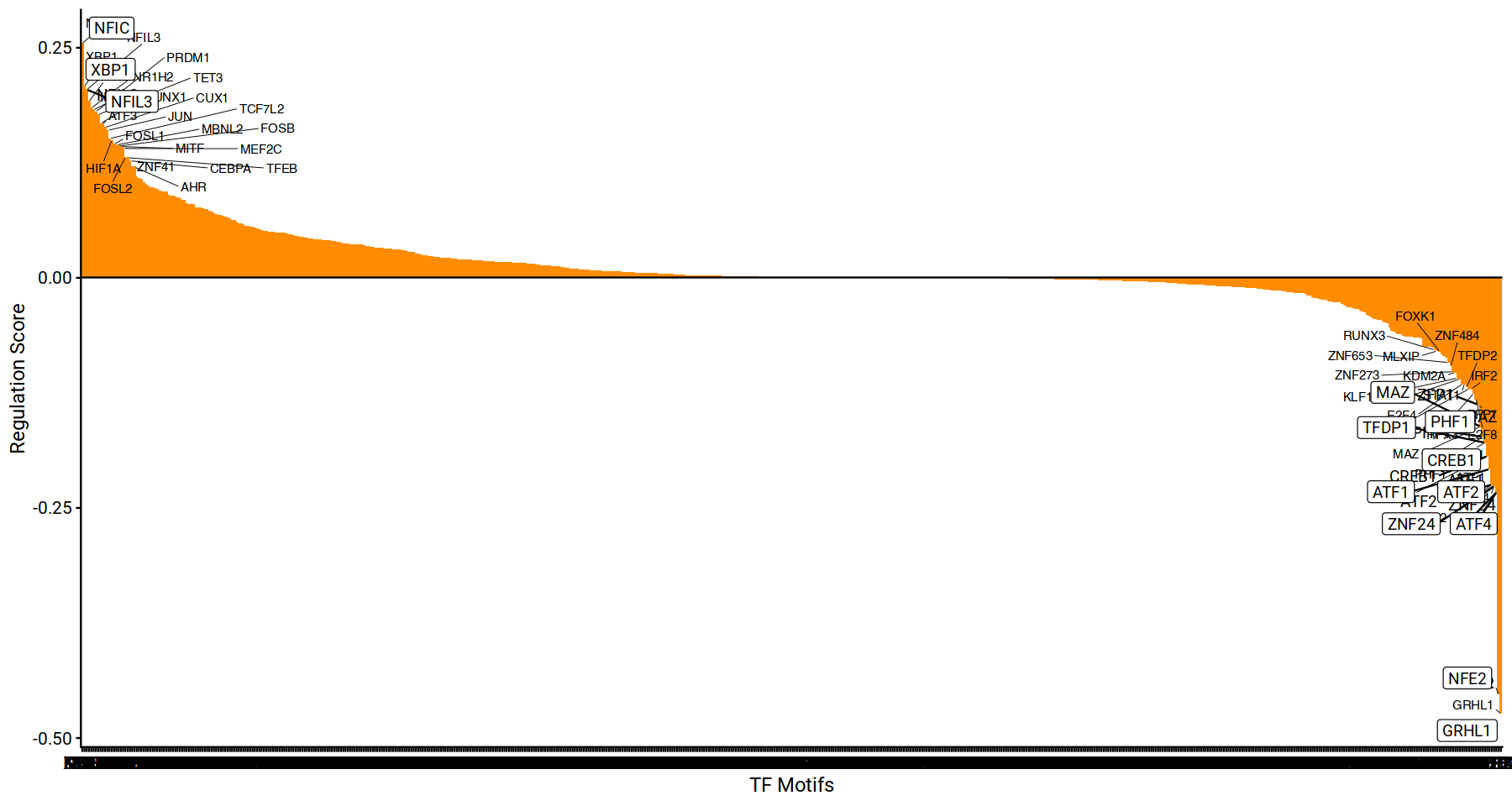
按平均调控分数对候选驱动 TF 排序,比较其正向和负向关联。
drivers <- rankDrivers(figR.d, rankBy = "meanScore",interactive = FALSE)
options(repr.plot.width=15, repr.plot.height=8)
drivers + geom_text_repel(family='roboto') + geom_label_repel(family='roboto') + cowplot::theme_cowplot(font_family='roboto') + labs(font_family='roboto')
Ranking TFs by mean regulation score across all DORCs ..
Warning message:
“ggrepel: 39 unlabeled data points (too many overlaps). Consider increasing max.overlaps”
Warning message:
“ggrepel: 51 unlabeled data points (too many overlaps). Consider increasing max.overlaps”
Warning message:
“ggrepel: 55 unlabeled data points (too many overlaps). Consider increasing max.overlaps”
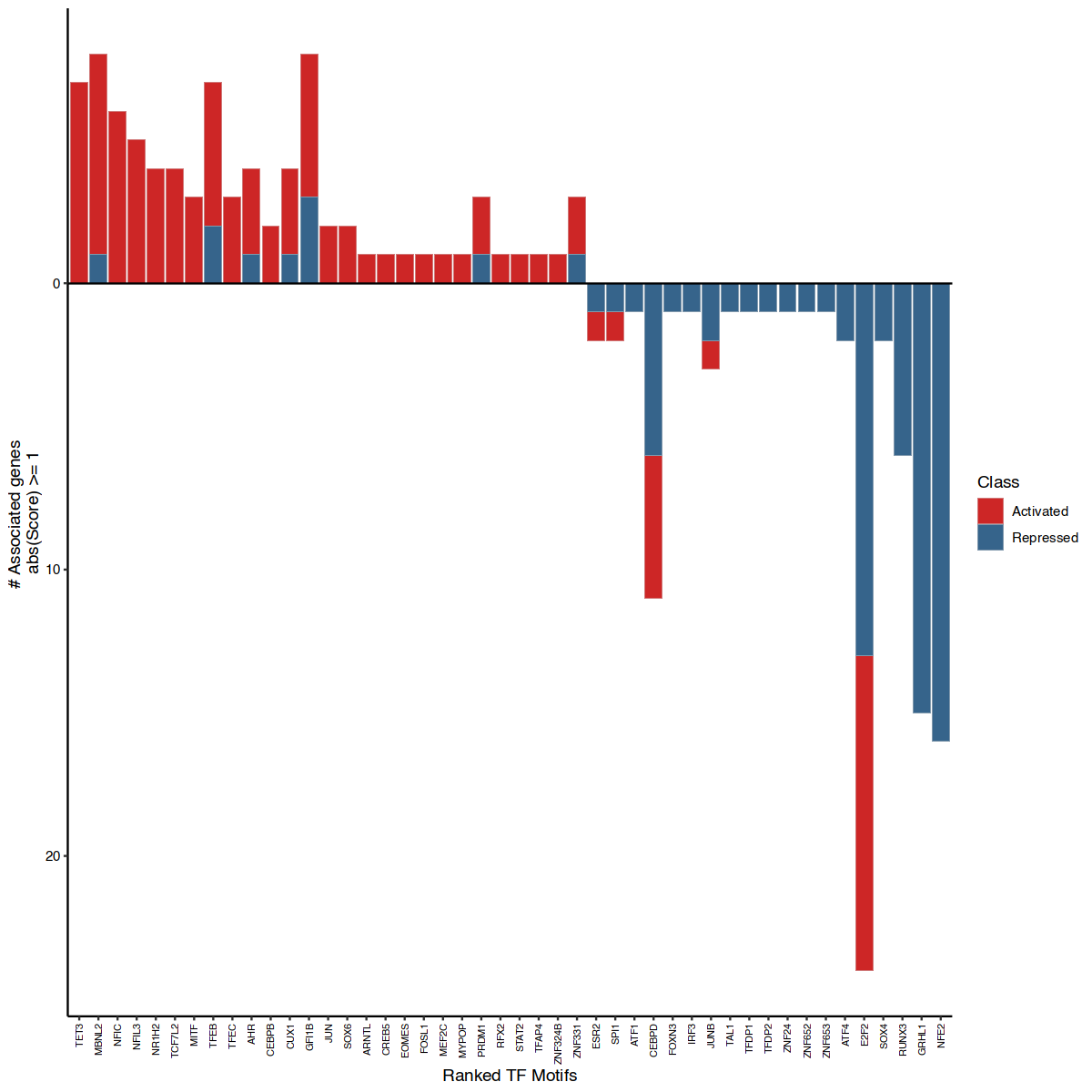
也可按超过评分阈值的潜在靶基因数量对 TF 基序排序,查看哪些候选因子可能参与较广泛的激活或抑制程序。这里的靶基因及作用方向均来自模型推断。
options(repr.plot.width=10, repr.plot.height=10)
rankDrivers(figR.d,score.cut = 1, rankBy = "nTargets", interactive = FALSE, fontsiz)
Ranking TFs by total number of associated DORCs ..
Using absolute score cut-off of: 1 ..
热图以靶基因为行、TF 为列,展示 TF–DORC 关联的综合调控分数。它与前面逐细胞计算的 DORC 可及性分数不同。
library(grid)
library(ComplexHeatmap)
options(repr.plot.width=10, repr.plot.height=10)
pushViewport(viewport(gp = gpar(fontfamily = "sans")));
heatmap <- plotfigRHeatmap(figR.d = figR.d,
score.cut = 1,
TFs = unique(figR.d$Motif),
column_names_gp = gpar(fontsize=10), # from ComplexHeatmap
show_row_dend = FALSE # from ComplexHeatmap
)
draw(heatmap, newpage = FALSE)
popViewport()
Using absolute score cut-off of: 1 ..


Using Score as value column: use value.var to override.

Plotting 45 DORCs x 46TFs
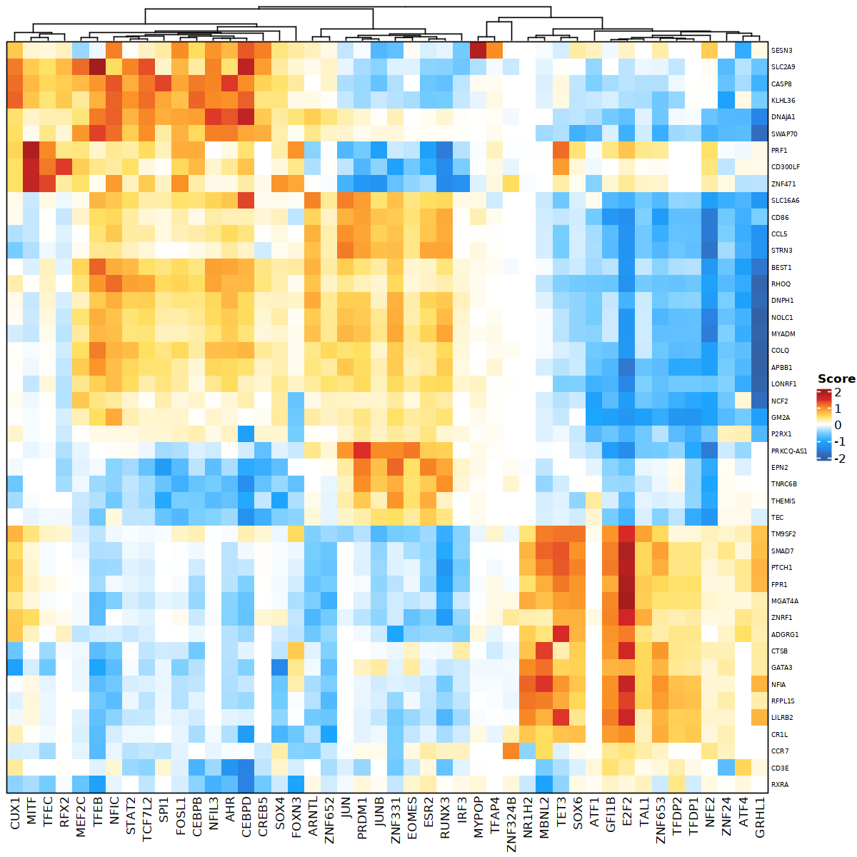
该图便于查看主要候选 TF 与潜在靶基因之间的关联模式。
最后,使用 networkD3 绘制关联网络,探索多个 TF 共享的靶基因,以及可能相互重叠的调节子(regulon),即某个 TF 及其候选靶基因集合。
library(networkD3)
library(r2d3)
library(imager)
# generate the network
d3 <- plotfigRNetwork(figR.d,
score.cut = 1,
TFs = unique(figR.d$Motif),
weight.edges = TRUE)# in a local session, the network can be manipulated interactively
d3将网络保存为 HTML 或 PNG
# If pandoc if not found by R, here the bin path in the environment has to be provided e.g. `envs/best_practices_regulons_rnanatac/bin`
# rmarkdown::find_pandoc(dir = "bin_path") # e.g. bin_path = '~/miniconda3/envs/best_practices_regulons_rnanatac/bin'

# is saved as an image and shown for exploratory purposes outside of this notebook
save_d3_html(
  d3,
  'network_tutorial_rna_n_atac.html',
)
# the network is saved as an image and shown for online purposes.
save_d3_png(
d3,
'network_tutorial_rna_n_atac.png',
width = 350,
height = 450,
delay = 4.0,
zoom = 1.6,
)im <- load.image('network_tutorial_rna_atac.png')
plot(im)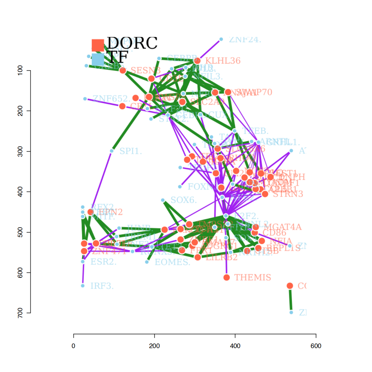
记录运行本笔记本时使用的软件包及版本。
sessionInfo()输出
R version 4.2.2 (2022-10-31)
Platform: x86_64-conda-linux-gnu (64-bit)
Running under: Ubuntu 20.04 LTS

Matrix products: default
BLAS/LAPACK: /home/rio/miniconda3/envs/best_practices_regulons_rnanatac/lib/libopenblasp-r0.3.21.so

locale:
 [1] LC_CTYPE=C.UTF-8       LC_NUMERIC=C           LC_TIME=C.UTF-8
 [4] LC_COLLATE=C.UTF-8     LC_MONETARY=C.UTF-8    LC_MESSAGES=C.UTF-8
 [7] LC_PAPER=C.UTF-8       LC_NAME=C              LC_ADDRESS=C
[10] LC_TELEPHONE=C         LC_MEASUREMENT=C.UTF-8 LC_IDENTIFICATION=C

attached base packages:
 [1] grid      parallel  stats4    stats     graphics  grDevices utils
 [8] datasets  methods   base

other attached packages:
 [1] imager_0.42.19                    magrittr_2.0.3
 [3] r2d3_0.2.6                        networkD3_0.4
 [5] ComplexHeatmap_2.14.0             BuenColors_0.5.6
 [7] MASS_7.3-58.3                     patchwork_1.1.2
 [9] ggrastr_1.0.1                     doParallel_1.0.17
[11] iterators_1.0.14                  foreach_1.5.2
[13] ggrepel_0.9.3                     BSgenome.Hsapiens.UCSC.hg38_1.4.5
[15] BSgenome_1.66.3                   rtracklayer_1.58.0
[17] Biostrings_2.66.0                 XVector_0.38.0
[19] FNN_1.1.3.2                       umap_0.2.10.0
[21] cisTopic_0.3.0                    SingleCellExperiment_1.20.0
[23] zellkonverter_1.8.0               FigR_0.1.0
[25] motifmatchr_1.20.0                chromVAR_1.20.0
[27] cowplot_1.1.1                     ggplot2_3.4.1
[29] dplyr_1.1.1                       SummarizedExperiment_1.28.0
[31] Biobase_2.58.0                    GenomicRanges_1.50.0
[33] GenomeInfoDb_1.34.9               IRanges_2.32.0
[35] S4Vectors_0.36.0                  BiocGenerics_0.44.0
[37] MatrixGenerics_1.10.0             matrixStats_0.63.0
[39] Matrix_1.5-3

loaded via a namespace (and not attached):
  [1] utf8_1.2.3                  reticulate_1.26
  [3] R.utils_2.12.2              tidyselect_1.2.0
  [5] poweRlaw_0.70.6             RSQLite_2.3.0
  [7] AnnotationDbi_1.60.2        htmlwidgets_1.6.2
  [9] gmp_0.7-1                   BiocParallel_1.32.5
 [11] munsell_0.5.0               codetools_0.2-19
 [13] DT_0.27                     pbdZMQ_0.3-9
 [15] miniUI_0.1.1.1              withr_2.5.0
 [17] RcisTarget_1.18.2           colorspace_2.1-0
 [19] filelock_1.0.2              knitr_1.42
 [21] uuid_1.1-0                  rstudioapi_0.14
 [23] pbmcapply_1.5.1             labeling_0.4.2
 [25] repr_1.1.6                  GenomeInfoDbData_1.2.9
 [27] lgr_0.4.4                   bit64_4.0.5
 [29] farver_2.1.1                rprojroot_2.0.3
 [31] basilisk_1.9.12             vctrs_0.6.1
 [33] generics_0.1.3              xfun_0.38
 [35] float_0.3-1                 R6_2.5.1
 [37] clue_0.3-64                 ggbeeswarm_0.7.1
 [39] bitops_1.0-7                arrow_10.0.1
 [41] cachem_1.0.7                DelayedArray_0.24.0
 [43] assertthat_0.2.1            promises_1.2.0.1
 [45] BiocIO_1.8.0                scales_1.2.1
 [47] beeswarm_0.4.0              gtable_0.3.3
 [49] Cairo_1.6-0                 processx_3.8.0
 [51] bmp_0.3                     seqLogo_1.64.0
 [53] rlang_1.1.0                 GlobalOptions_0.1.2
 [55] text2vec_0.6.3              splines_4.2.2
 [57] lazyeval_0.2.2              yaml_2.3.7
 [59] reshape2_1.4.4              httpuv_1.6.9
 [61] tools_4.2.2                 feather_0.3.5
 [63] nabor_0.5.0                 gplots_3.1.3
 [65] ellipsis_0.3.2              RColorBrewer_1.1-3
 [67] Rcpp_1.0.10                 plyr_1.8.8
 [69] base64enc_0.1-3             sparseMatrixStats_1.10.0
 [71] zlibbioc_1.44.0             purrr_1.0.1
 [73] RCurl_1.98-1.10             ps_1.7.3
 [75] basilisk.utils_1.10.0       openssl_2.0.5
 [77] GetoptLong_1.0.5            cluster_2.1.4
 [79] here_1.0.1                  data.table_1.14.8
 [81] RSpectra_0.16-1             readbitmap_0.1.5
 [83] circlize_0.4.15             mlapi_0.1.1
 [85] fitdistrplus_1.1-8          hms_1.1.3
 [87] mime_0.12                   evaluate_0.20
 [89] xtable_1.8-4                RhpcBLASctl_0.23-42
 [91] XML_3.99-0.14               jpeg_0.1-10
 [93] AUCell_1.20.2               shape_1.4.6
 [95] compiler_4.2.2              tibble_3.2.1
 [97] KernSmooth_2.23-20          crayon_1.5.2
 [99] R.oo_1.25.0                 htmltools_0.5.5
[101] tiff_0.1-11                 later_1.3.0
[103] tzdb_0.3.0                  TFBSTools_1.36.0
[105] snow_0.4-4                  tidyr_1.3.0
[107] DBI_1.1.3                   readr_2.1.4
[109] cli_3.6.1                   R.methodsS3_1.8.2
[111] igraph_1.4.1                pkgconfig_2.0.3
[113] GenomicAlignments_1.34.0    rsparse_0.5.1
[115] dir.expiry_1.6.0            TFMPvalue_0.0.9
[117] IRdisplay_1.1               plotly_4.10.1
[119] annotate_1.76.0             lda_1.4.2
[121] vipor_0.4.5                 DirichletMultinomial_1.40.0
[123] webshot_0.5.4               callr_3.7.3
[125] stringr_1.5.0               digest_0.6.31
[127] pracma_2.4.2                CNEr_1.34.0
[129] graph_1.76.0                rmarkdown_2.21
[131] DelayedMatrixStats_1.20.0   GSEABase_1.60.0
[133] restfulr_0.0.15             shiny_1.7.4
[135] Rsamtools_2.14.0            gtools_3.9.4
[137] rjson_0.2.21                lifecycle_1.0.3
[139] jsonlite_1.8.4              viridisLite_0.4.1
[141] askpass_1.1                 fansi_1.0.4
[143] pillar_1.9.0                lattice_0.20-45
[145] KEGGREST_1.38.0             fastmap_1.1.1
[147] httr_1.4.5                  survival_3.5-5
[149] GO.db_3.16.0                glue_1.6.2
[151] png_0.1-8                   bit_4.0.5
[153] stringi_1.7.12              blob_1.2.4
[155] doSNOW_1.0.20               caTools_1.18.2
[157] memoise_2.0.1               Rmpfr_0.9-1
[159] IRkernel_1.3.2 测验
理论
FigR
- Spitz, F., & Furlong, E. E. M. (2012). Transcription factors: from enhancer binding to developmental control. Nat. Rev. Genet., 13(9), 613–626.
- Kartha, V. K., Duarte, F. M., Hu, Y., Ma, S., Chew, J. G., Lareau, C. A., Earl, A., Burkett, Z. D., Kohlway, A. S., Lebofsky, R., & Buenrostro, J. D. (2022). Functional inference of gene regulation using single-cell multi-omics. Cell Genom, 2(9).
- Bravo González-Blas, C., Minnoye, L., Papasokrati, D., Aibar, S., Hulselmans, G., Christiaens, V., Davie, K., Wouters, J., & Aerts, S. (2019). cisTopic: cis-regulatory topic modeling on single-cell ATAC-seq data. Nat. Methods, 16(5), 397–400.
- Schep, A. N., Wu, B., Buenrostro, J. D., & Greenleaf, W. J. (2017). chromVAR: inferring transcription-factor-associated accessibility from single-cell epigenomic data. Nat. Methods, 14(10), 975–978.