🧠 关键要点
现代单细胞实验常同时测量多种模态(modality),例如 RNA、转座酶可及染色质测定(assay for transposase-accessible chromatin, ATAC) 和蛋白质。AnnData 面向单模态(unimodal)数据,而多模态实验(multimodal experiment)则需要 MuData 这类可组织多个数据集的容器。
一个 MuData 对象可存储多个 AnnData 对象(每种模态对应一个),同时共享细胞和 feature 的全局注释。该结构既支持模态特异性分析,也支持在同一数据集中开展联合多模态计算(joint multimodal computation)。
muon 框架扩展了分析生态,提供针对 RNA 之外其他模态(如 ATAC 或蛋白质数据)的预处理和分析工具,并包含跨模态整合(multimodal integration)信息的方法。
空间组学(spatial omics)技术在测量分子数据的同时保留组织内的空间信息(spatial context)。SpatialData 数据结构把图像、坐标、几何对象和分子测量统一存储在一起。
Squidpy 将分子谱与空间信息结合起来,同时提供分析和可视化工具。它构建于 Scanpy 和 AnnData 之上,保留了模块化与可扩展性。
⚙️ 环境设置
安装 conda:
在创建环境之前,请确保 conda 已安装在您的系统中。
保存 yml 内容:
将 yml 选项卡中的内容复制到名为
environment.yml。
创建环境:
打开终端或命令提示符。
运行以下命令:
conda env create -f environment.yml
激活环境:
创建好环境后,使用以下命令激活它:
conda activate <environment_name>请将
<environment_name>替换为environment.yml文件中指定的环境名称。该名称在 yml 文件中如下所示:name: <environment_name>
验证安装:
通过运行以下命令,检查环境是否创建成功:
conda env list
name: advanced_data_structures_and_frameworks
channels:
  - conda-forge
  - bioconda
dependencies:
  - conda-forge::imagecodecs<2026,>=2025.8.2
  - conda-forge::muon=0.1.7
  - conda-forge::python=3.12.12
  - conda-forge::squidpy=1.8.1
  - conda-forge::scanpy=1.12
  - conda-forge::leidenalg=0.11.0
  - conda-forge::python-igraph=1.0.0
  - pip
  - pip:
      - lamindb
      - pysam==0.23.3
🗄️ 获取数据和笔记本
本书使用 lamindb 来存储、共享和加载数据集与笔记本,所用实例为 theislab/sc-best-practices 实例。我们感谢以下平台提供的免费托管:Lamin Labs。
安装 lamindb
安装 lamindb Python 软件包:
pip install lamindb可选择创建 Lamin 账户
请按照 相关说明注册并登录
验证你的设置
运行
lamin connect命令:
import lamindb as ln

ln.Artifact.connect("theislab/sc-best-practices").df()
你现在应该能看到最多 100 个已存储的数据集。
访问数据集(Artifact)
在以下页面搜索数据集:Artifacts 页面
加载一个 Artifact 及其对应的对象:
import lamindb as ln
af = ln.Artifact.connect("theislab/sc-best-practices").get(key="key_of_dataset", is_latest=True)
obj = af.load()
该对象现在已可在内存中访问,并可用于分析。请调整
lamindb.Artifact.connect("theislab/sc-best-practices").get("SOMEIDXXXX")后缀,以获取相应版本。访问笔记本(Transform)
在以下页面搜索笔记本:Transforms 页面
加载笔记本:
lamin load <notebook url>该命令会将笔记本下载到当前工作目录。与
Artifacts类似,你也可以调整后缀 ID 来获取旧版本。
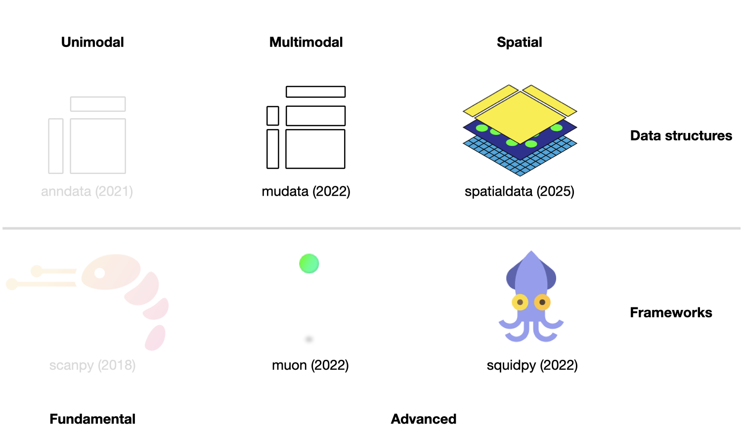
图 1:scverse 生态系统概览,突出显示本章涉及的库。括号内标注了各库被科学期刊发表的日期。各库的图标取自相应的 GitHub 页面 Virshup et al., 2021Wolf et al., 2018Bredikhin et al., 2022Palla et al., 2022Marconato et al., 2025。
本章假定读者已经熟悉 AnnData 和 scanpy(参见 上一章)。它进一步引入两种数据结构——用于多模态实验的 MuData 和用于空间分辨数据的 SpatialData——以及构建在各自之上的分析框架。
使用 MuData 存储多模态数据
AnnData 主要用于存储和操作单模态(unimodal)数据。然而,通过测序进行转录组与表位索引(cellular indexing of transcriptomes and epitopes by sequencing, CITE-seq) 等多模态实验会通过同时测量 RNA 和表面蛋白来产生多模态数据。这类数据需要更高级的存储方式,而这正是 MuData 发挥作用的地方。MuData 构建在 AnnData 之上,用于存储和操作多模态数据。Muon Bredikhin et al., 2022,作为“scanpy 的对应物”和 scverse 的核心包,随后可用于分析多模态组学数据。下一节的内容基于 MuData 快速入门 和 多模态数据对象 教程。
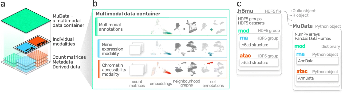
图 2:MuData 概览。图片取自 Bredikhin et al., 2022。
安装
MuData 可在 PyPI 和 Conda 上获取,可使用以下任一命令安装。
pip install mudata
conda install -c conda-forge mudata
MuData 背后的主要思想是:MuData 对象包含对各单模态数据所对应的单个 AnnData 对象的引用,但 MuData 对象本身也存储多模态注释。因此,既可以直接访问这些 AnnData 对象,对单模态数据做变换并把结果存进相应的 AnnData 注释中;也可以把各模态聚合起来做联合计算,并把结果存进全局的 MuData 对象。从技术上讲,这是通过 MuData 对象实现的:它在表示模态(modality)的 .mod 属性中包含一个由 AnnData 对象组成的字典,每个模态对应一个。与 AnnData 对象本身一样,MuData 对象也包含诸如 .obs 等属性(用于存放对观测(样本或细胞)的注释),以及诸如 .obsm 等属性(用于存放嵌入(embedding)等多维注释)。
初始化 MuData 对象
让我们从 mudata 包中导入 MuData。
import lamindb as ln
import mudata as md
import numpy as np

ln.track()
输出
→ loaded Transform('em2cp9S0T9WE0000', key='advanced_data_structures_and_frameworks.ipynb'), re-started Run('aAHUPh3azE6M2eum') at 2026-03-05 06:13:20 UTC
→ notebook imports: lamindb==2.0.1 mudata==0.3.3 muon==0.1.7 numpy==2.4.2 scanpy==1.11.5 scikit-learn==1.8.0 spatialdata-plot==0.2.14 spatialdata==0.6.1 squidpy==1.7.0
• recommendation: to identify the notebook across renames, pass the uid: ln.track("em2cp9S0T9WE")
要创建一个示例 MuData 对象,我们需要模拟数据。因此,我们创建了两个 AnnData 对象,它们包含 针对相同观测的数据,但针对 不同变量。
adata = ln.Artifact.get(
    key="introduction/advanced_data_structures_and_frameworks_mudata_1.h5ad",
).load()
adata
AnnData object with n_obs × n_vars = 1000 × 100adata2 = ln.Artifact.get(
key="introduction/advanced_data_structures_and_frameworks_mudata_2.h5ad",
).load()
adata2AnnData object with n_obs × n_vars = 1000 × 50随后,可以把这两个 AnnData 对象(两个“模态”)封装进一个 MuData 对象中。这里,第一个模态称为 A,第二个称为 B。
mdata = md.MuData({"A": adata, "B": adata2})
mdata对于 MuData 对象,其观测和变量都是全局的,这意味着同名的观测(.obs_names)在不同模态中被视为同一个观测(例如 obs_1 属于 adata 和 obs_1 属于 adata2)。这也意味着变量名(.var_names)应当是唯一的(例如 var_1 属于 adata 和 var2_1 属于 adata2)。这反映在上述对象描述中:mdata 有 1000 个观测和 150(=100+50)个变量。
MuData 属性
.mod
MuData 对象除了包含此前介绍的 AnnData 注释,例如 .obs 或 .var,还增加了 .mod,用于访问各个模态。各模态存储在一个集合中,可通过 MuData 对象的 .mod 属性来访问,其中以模态名称为键、AnnData 对象为值。
list(mdata.mod.keys())['A', 'B']可以通过各模态的名称,借助 .mod 属性来访问单个模态,也可以直接通过 MuData 对象本身作为简写来访问。
print(mdata.mod["A"])
print(mdata["A"])
AnnData object with n_obs × n_vars = 1000 × 100
AnnData object with n_obs × n_vars = 1000 × 100
.obs 和 .var
样本(细胞)注释可通过 .obs 属性访问,默认包含各个模态 .obs DataFrame 中相应列的副本;.var 则包含变量(特征)注释。从单个模态复制来的观测列以模态名为前缀,例如 rna:n_genes;变量列同样如此。但是,如果多个模态的 .var 中存在同名列(例如 n_cells),这些列会跨模态合并且不添加前缀。当各模态 AnnData 对象中的这些槽位发生变化时(例如新增列或筛除样本/细胞),必须调用 .update() 方法同步这些变化(见下文)。
mdata.var_namesIndex(['var_1', 'var_2', 'var_3', 'var_4', 'var_5', 'var_6', 'var_7', 'var_8',
'var_9', 'var_10',
...
'var2_41', 'var2_42', 'var2_43', 'var2_44', 'var2_45', 'var2_46',
'var2_47', 'var2_48', 'var2_49', 'var2_50'],
dtype='object', length=150)样本(细胞)的多维注释可在 .obsm 属性中访问。例如,它可以是在所有模态上联合学习得到的 统一流形近似与投影(uniform manifold approximation and projection, UMAP) 坐标。
如果模态形状发生变化(例如更改 var_names),需运行 MuData.update(),才能把相应更新同步到 MuData 对象。
adata2.var_names = ["var_ad2_" + e.split("_")[1] for e in adata2.var_names]
print("Outdated variables names: ...,", ", ".join(mdata.var_names[-3:]))
mdata.update()
print("Updated variables names: ...,", ", ".join(mdata.var_names[-3:]))
Outdated variables names: ..., var2_48, var2_49, var2_50
Updated variables names: ..., var_ad2_48, var_ad2_49, var_ad2_50
需要特别注意的是,各个模态以指向原始对象的引用形式存储。因此,若原始 AnnData 发生变化,该变化也会反映在 MuData 对象中。
# Add some unstructured data to the original object
adata.uns["misc"] = {"adata": True}
# Access modality A via the .mod attribute
mdata.mod["A"].uns["misc"]{'adata': True}变量映射
在构建 MuData 对象时,会在观测与各个模态之间、以及变量与各个模态之间创建一个全局的二值映射。由于在 mdata 中,各模态的所有观测都相同,因此观测映射中的所有值都被设为 True。
mdata.obsm["A"]输出
array([[ True],
[ True],
[ True],
[ True],
[ True],
[ True],
[ True],
[ True],
[ True],
[ True],
[ True],
[ True],
[ True],
[ True],
[ True],
[ True],
[ True],
[ True],
[ True],
[ True],
[ True],
[ True],
[ True],
[ True],
[ True],
[ True],
[ True],
[ True],
[ True],
[ True],
[ True],
[ True],
[ True],
[ True],
[ True],
[ True],
[ True],
[ True],
[ True],
[ True],
[ True],
[ True],
[ True],
[ True],
[ True],
[ True],
[ True],
[ True],
[ True],
[ True],
[ True],
[ True],
[ True],
[ True],
[ True],
[ True],
[ True],
[ True],
[ True],
[ True],
[ True],
[ True],
[ True],
[ True],
[ True],
[ True],
[ True],
[ True],
[ True],
[ True],
[ True],
[ True],
[ True],
[ True],
[ True],
[ True],
[ True],
[ True],
[ True],
[ True],
[ True],
[ True],
[ True],
[ True],
[ True],
[ True],
[ True],
[ True],
[ True],
[ True],
[ True],
[ True],
[ True],
[ True],
[ True],
[ True],
[ True],
[ True],
[ True],
[ True],
[ True],
[ True],
[ True],
[ True],
[ True],
[ True],
[ True],
[ True],
[ True],
[ True],
[ True],
[ True],
[ True],
[ True],
[ True],
[ True],
[ True],
[ True],
[ True],
[ True],
[ True],
[ True],
[ True],
[ True],
[ True],
[ True],
[ True],
[ True],
[ True],
[ True],
[ True],
[ True],
[ True],
[ True],
[ True],
[ True],
[ True],
[ True],
[ True],
[ True],
[ True],
[ True],
[ True],
[ True],
[ True],
[ True],
[ True],
[ True],
[ True],
[ True],
[ True],
[ True],
[ True],
[ True],
[ True],
[ True],
[ True],
[ True],
[ True],
[ True],
[ True],
[ True],
[ True],
[ True],
[ True],
[ True],
[ True],
[ True],
[ True],
[ True],
[ True],
[ True],
[ True],
[ True],
[ True],
[ True],
[ True],
[ True],
[ True],
[ True],
[ True],
[ True],
[ True],
[ True],
[ True],
[ True],
[ True],
[ True],
[ True],
[ True],
[ True],
[ True],
[ True],
[ True],
[ True],
[ True],
[ True],
[ True],
[ True],
[ True],
[ True],
[ True],
[ True],
[ True],
[ True],
[ True],
[ True],
[ True],
[ True],
[ True],
[ True],
[ True],
[ True],
[ True],
[ True],
[ True],
[ True],
[ True],
[ True],
[ True],
[ True],
[ True],
[ True],
[ True],
[ True],
[ True],
[ True],
[ True],
[ True],
[ True],
[ True],
[ True],
[ True],
[ True],
[ True],
[ True],
[ True],
[ True],
[ True],
[ True],
[ True],
[ True],
[ True],
[ True],
[ True],
[ True],
[ True],
[ True],
[ True],
[ True],
[ True],
[ True],
[ True],
[ True],
[ True],
[ True],
[ True],
[ True],
[ True],
[ True],
[ True],
[ True],
[ True],
[ True],
[ True],
[ True],
[ True],
[ True],
[ True],
[ True],
[ True],
[ True],
[ True],
[ True],
[ True],
[ True],
[ True],
[ True],
[ True],
[ True],
[ True],
[ True],
[ True],
[ True],
[ True],
[ True],
[ True],
[ True],
[ True],
[ True],
[ True],
[ True],
[ True],
[ True],
[ True],
[ True],
[ True],
[ True],
[ True],
[ True],
[ True],
[ True],
[ True],
[ True],
[ True],
[ True],
[ True],
[ True],
[ True],
[ True],
[ True],
[ True],
[ True],
[ True],
[ True],
[ True],
[ True],
[ True],
[ True],
[ True],
[ True],
[ True],
[ True],
[ True],
[ True],
[ True],
[ True],
[ True],
[ True],
[ True],
[ True],
[ True],
[ True],
[ True],
[ True],
[ True],
[ True],
[ True],
[ True],
[ True],
[ True],
[ True],
[ True],
[ True],
[ True],
[ True],
[ True],
[ True],
[ True],
[ True],
[ True],
[ True],
[ True],
[ True],
[ True],
[ True],
[ True],
[ True],
[ True],
[ True],
[ True],
[ True],
[ True],
[ True],
[ True],
[ True],
[ True],
[ True],
[ True],
[ True],
[ True],
[ True],
[ True],
[ True],
[ True],
[ True],
[ True],
[ True],
[ True],
[ True],
[ True],
[ True],
[ True],
[ True],
[ True],
[ True],
[ True],
[ True],
[ True],
[ True],
[ True],
[ True],
[ True],
[ True],
[ True],
[ True],
[ True],
[ True],
[ True],
[ True],
[ True],
[ True],
[ True],
[ True],
[ True],
[ True],
[ True],
[ True],
[ True],
[ True],
[ True],
[ True],
[ True],
[ True],
[ True],
[ True],
[ True],
[ True],
[ True],
[ True],
[ True],
[ True],
[ True],
[ True],
[ True],
[ True],
[ True],
[ True],
[ True],
[ True],
[ True],
[ True],
[ True],
[ True],
[ True],
[ True],
[ True],
[ True],
[ True],
[ True],
[ True],
[ True],
[ True],
[ True],
[ True],
[ True],
[ True],
[ True],
[ True],
[ True],
[ True],
[ True],
[ True],
[ True],
[ True],
[ True],
[ True],
[ True],
[ True],
[ True],
[ True],
[ True],
[ True],
[ True],
[ True],
[ True],
[ True],
[ True],
[ True],
[ True],
[ True],
[ True],
[ True],
[ True],
[ True],
[ True],
[ True],
[ True],
[ True],
[ True],
[ True],
[ True],
[ True],
[ True],
[ True],
[ True],
[ True],
[ True],
[ True],
[ True],
[ True],
[ True],
[ True],
[ True],
[ True],
[ True],
[ True],
[ True],
[ True],
[ True],
[ True],
[ True],
[ True],
[ True],
[ True],
[ True],
[ True],
[ True],
[ True],
[ True],
[ True],
[ True],
[ True],
[ True],
[ True],
[ True],
[ True],
[ True],
[ True],
[ True],
[ True],
[ True],
[ True],
[ True],
[ True],
[ True],
[ True],
[ True],
[ True],
[ True],
[ True],
[ True],
[ True],
[ True],
[ True],
[ True],
[ True],
[ True],
[ True],
[ True],
[ True],
[ True],
[ True],
[ True],
[ True],
[ True],
[ True],
[ True],
[ True],
[ True],
[ True],
[ True],
[ True],
[ True],
[ True],
[ True],
[ True],
[ True],
[ True],
[ True],
[ True],
[ True],
[ True],
[ True],
[ True],
[ True],
[ True],
[ True],
[ True],
[ True],
[ True],
[ True],
[ True],
[ True],
[ True],
[ True],
[ True],
[ True],
[ True],
[ True],
[ True],
[ True],
[ True],
[ True],
[ True],
[ True],
[ True],
[ True],
[ True],
[ True],
[ True],
[ True],
[ True],
[ True],
[ True],
[ True],
[ True],
[ True],
[ True],
[ True],
[ True],
[ True],
[ True],
[ True],
[ True],
[ True],
[ True],
[ True],
[ True],
[ True],
[ True],
[ True],
[ True],
[ True],
[ True],
[ True],
[ True],
[ True],
[ True],
[ True],
[ True],
[ True],
[ True],
[ True],
[ True],
[ True],
[ True],
[ True],
[ True],
[ True],
[ True],
[ True],
[ True],
[ True],
[ True],
[ True],
[ True],
[ True],
[ True],
[ True],
[ True],
[ True],
[ True],
[ True],
[ True],
[ True],
[ True],
[ True],
[ True],
[ True],
[ True],
[ True],
[ True],
[ True],
[ True],
[ True],
[ True],
[ True],
[ True],
[ True],
[ True],
[ True],
[ True],
[ True],
[ True],
[ True],
[ True],
[ True],
[ True],
[ True],
[ True],
[ True],
[ True],
[ True],
[ True],
[ True],
[ True],
[ True],
[ True],
[ True],
[ True],
[ True],
[ True],
[ True],
[ True],
[ True],
[ True],
[ True],
[ True],
[ True],
[ True],
[ True],
[ True],
[ True],
[ True],
[ True],
[ True],
[ True],
[ True],
[ True],
[ True],
[ True],
[ True],
[ True],
[ True],
[ True],
[ True],
[ True],
[ True],
[ True],
[ True],
[ True],
[ True],
[ True],
[ True],
[ True],
[ True],
[ True],
[ True],
[ True],
[ True],
[ True],
[ True],
[ True],
[ True],
[ True],
[ True],
[ True],
[ True],
[ True],
[ True],
[ True],
[ True],
[ True],
[ True],
[ True],
[ True],
[ True],
[ True],
[ True],
[ True],
[ True],
[ True],
[ True],
[ True],
[ True],
[ True],
[ True],
[ True],
[ True],
[ True],
[ True],
[ True],
[ True],
[ True],
[ True],
[ True],
[ True],
[ True],
[ True],
[ True],
[ True],
[ True],
[ True],
[ True],
[ True],
[ True],
[ True],
[ True],
[ True],
[ True],
[ True],
[ True],
[ True],
[ True],
[ True],
[ True],
[ True],
[ True],
[ True],
[ True],
[ True],
[ True],
[ True],
[ True],
[ True],
[ True],
[ True],
[ True],
[ True],
[ True],
[ True],
[ True],
[ True],
[ True],
[ True],
[ True],
[ True],
[ True],
[ True],
[ True],
[ True],
[ True],
[ True],
[ True],
[ True],
[ True],
[ True],
[ True],
[ True],
[ True],
[ True],
[ True],
[ True],
[ True],
[ True],
[ True],
[ True],
[ True],
[ True],
[ True],
[ True],
[ True],
[ True],
[ True],
[ True],
[ True],
[ True],
[ True],
[ True],
[ True],
[ True],
[ True],
[ True],
[ True],
[ True],
[ True],
[ True],
[ True],
[ True],
[ True],
[ True],
[ True],
[ True],
[ True],
[ True],
[ True],
[ True],
[ True],
[ True],
[ True],
[ True],
[ True],
[ True],
[ True],
[ True],
[ True],
[ True],
[ True],
[ True],
[ True],
[ True],
[ True],
[ True],
[ True],
[ True],
[ True],
[ True],
[ True],
[ True],
[ True],
[ True],
[ True],
[ True],
[ True],
[ True],
[ True],
[ True],
[ True],
[ True],
[ True],
[ True],
[ True],
[ True],
[ True],
[ True],
[ True],
[ True],
[ True],
[ True],
[ True],
[ True],
[ True],
[ True],
[ True],
[ True],
[ True],
[ True],
[ True],
[ True],
[ True],
[ True],
[ True],
[ True],
[ True],
[ True],
[ True],
[ True],
[ True],
[ True],
[ True],
[ True],
[ True],
[ True],
[ True],
[ True],
[ True],
[ True],
[ True],
[ True],
[ True],
[ True],
[ True],
[ True],
[ True],
[ True],
[ True],
[ True],
[ True],
[ True],
[ True],
[ True],
[ True],
[ True],
[ True],
[ True],
[ True],
[ True],
[ True],
[ True],
[ True],
[ True],
[ True],
[ True],
[ True],
[ True],
[ True],
[ True],
[ True],
[ True],
[ True],
[ True],
[ True],
[ True],
[ True],
[ True],
[ True],
[ True],
[ True],
[ True],
[ True],
[ True],
[ True],
[ True],
[ True],
[ True],
[ True],
[ True],
[ True],
[ True],
[ True],
[ True],
[ True],
[ True],
[ True],
[ True],
[ True],
[ True],
[ True],
[ True],
[ True],
[ True],
[ True],
[ True],
[ True],
[ True],
[ True],
[ True],
[ True],
[ True],
[ True],
[ True],
[ True],
[ True],
[ True],
[ True],
[ True],
[ True],
[ True],
[ True]])np.sum(mdata.obsm["A"]) == np.sum(mdata.obsm["B"]) == 1000np.True_不过对于变量,这些映射是长度为 150 的向量。A 模态有 100 个 True 值,随后是 50 个 False 值。
mdata.varm["A"]输出
array([[ True],
       [ True],
       [ True],
       [ True],
       [ True],
       [ True],
       [ True],
       [ True],
       [ True],
       [ True],
       [ True],
       [ True],
       [ True],
       [ True],
       [ True],
       [ True],
       [ True],
       [ True],
       [ True],
       [ True],
       [ True],
       [ True],
       [ True],
       [ True],
       [ True],
       [ True],
       [ True],
       [ True],
       [ True],
       [ True],
       [ True],
       [ True],
       [ True],
       [ True],
       [ True],
       [ True],
       [ True],
       [ True],
       [ True],
       [ True],
       [ True],
       [ True],
       [ True],
       [ True],
       [ True],
       [ True],
       [ True],
       [ True],
       [ True],
       [ True],
       [ True],
       [ True],
       [ True],
       [ True],
       [ True],
       [ True],
       [ True],
       [ True],
       [ True],
       [ True],
       [ True],
       [ True],
       [ True],
       [ True],
       [ True],
       [ True],
       [ True],
       [ True],
       [ True],
       [ True],
       [ True],
       [ True],
       [ True],
       [ True],
       [ True],
       [ True],
       [ True],
       [ True],
       [ True],
       [ True],
       [ True],
       [ True],
       [ True],
       [ True],
       [ True],
       [ True],
       [ True],
       [ True],
       [ True],
       [ True],
       [ True],
       [ True],
       [ True],
       [ True],
       [ True],
       [ True],
       [ True],
       [ True],
       [ True],
       [ True],
       [False],
       [False],
       [False],
       [False],
       [False],
       [False],
       [False],
       [False],
       [False],
       [False],
       [False],
       [False],
       [False],
       [False],
       [False],
       [False],
       [False],
       [False],
       [False],
       [False],
       [False],
       [False],
       [False],
       [False],
       [False],
       [False],
       [False],
       [False],
       [False],
       [False],
       [False],
       [False],
       [False],
       [False],
       [False],
       [False],
       [False],
       [False],
       [False],
       [False],
       [False],
       [False],
       [False],
       [False],
       [False],
       [False],
       [False],
       [False],
       [False],
       [False]])
MuData 视图
与 AnnData 对象的行为类似,对 MuData 对象切片会返回原始数据的视图(view)。
view = mdata[:100, :1000]
print(view.is_view)
print(view["A"].is_view)
True
True
对 MuData 对象进行取子集(subsetting)很特殊,因为它会跨各个模态进行切片。例如,对一组 obs_names 和/或 var_names 进行的切片操作会在每个模态上执行,而不仅仅作用于全局的多模态注释。这种行为使工作流程很省内存,在处理大型数据集时尤为重要。不过,如果要修改该对象,就应当为它创建一个副本——副本不再是视图,也不再依赖于原始对象。
mdata_sub = view.copy()
mdata_sub.is_viewFalse共有观测
虽然 MuData 对象在两种模态上由相同的观测组成,但在现实世界中并非总是如此,有些数据可能缺失。在设计上,MuData 已考虑到这些情形,因为对于一个 MuData 实例而言,并不能保证各模态的观测相同(甚至相交)。值得注意的是,其他工具可能为处理缺失数据的某些常见情形提供便捷函数,例如 intersect_obs(),它在 muon 中实现。
MuData 对象的读写
与 AnnData 对象类似,MuData 对象被设计为可序列化为基于 层次化数据格式第 5 版(Hierarchical Data Format version 5, HDF5) 的 .h5mu 文件。所有模态都以各自的名称存储在 /mod HDF5 组中(该组位于 .h5mu 文件中)。每一个单独的模态,例如 /mod/A,其存储方式与它单独存储于 .h5ad 文件中时相同。MuData 对象可读写如下:
mdata.write("my_mudata.h5mu")
mdata_r = md.read("my_mudata.h5mu", backed=True)
mdata_r各个模态同样以 backed 模式存储在 .h5mu 文件中。
mdata_r["A"].isbackedTrue如果原始对象处于 backed 模式,请为 .copy() 调用提供一个新文件名,这样得到的对象就会在新位置以 backed 模式存储。
mdata_sub = mdata_r.copy("mdata_sub.h5mu")
print(mdata_sub.is_view)
print(mdata_sub.isbacked)
False
True
多模态方法
准备好 MuData 对象后,就可以使用多模态方法分析其中的数据。最简单直接的做法是拼接多个模态的矩阵,再执行降维(dimensionality reduction)等分析。
x = np.hstack([mdata.mod["A"].X, mdata.mod["B"].X])
x.shape
(1000, 150)我们可以编写一个简单的函数,对这样一个拼接后的矩阵运行 主成分分析(principal component analysis, PCA)。MuData 对象提供了一处用于存储多模态 嵌入:MuData .obsm。这类似于在各个单独模态上生成的嵌入的存储方式,只不过这次它保存在 MuData 对象内部,而不是 AnnData 的 .obsm。
例如,要对各模态的联合数值计算 PCA,可以将各模态中存储的数值按水平方向拼接,再对拼接后的矩阵执行 PCA。之所以可行,是因为各模态的观测数量一致;请记住,各模态的特征数量不必一致。
def simple_pca(mdata):
    from sklearn import decomposition

    x = np.hstack([m.X for m in mdata.mod.values()])

    pca = decomposition.PCA(n_components=2)
    components = pca.fit_transform(x)

    # By default, methods operate in-place and embeddings are stored in the .obsm slot
    mdata.obsm["X_pca"] = components
simple_pca(mdata)
print(mdata)MuData object with n_obs × n_vars = 1000 × 150
obsm: 'X_pca'
2 modalities
A: 1000 x 100
uns: 'misc'
B: 1000 x 50
我们计算得到的主成分现在存储在 MuData 对象本身之中,可供进一步的多模态变换使用。
然而在现实中,不同模态的特征往往来自不同的生成过程,因而不能直接比较,这时就需要专门的多模态整合(multimodal integration)方法。在组学领域,它们通常称为多组学(multi-omics)整合方法。下一节将介绍 muon:它不仅提供 RNA-seq 以外各类单模态数据的预处理工具,也提供多组学整合方法。
使用 muon 进行多模态数据分析
虽然 scanpy 提供 PCA、UMAP 和多种可视化等通用工具,但它主要面向 RNA-seq 数据。muon 填补了这一空白,为转座酶可及染色质测定(assay for transposase-accessible chromatin, ATAC) 测得的染色质可及性(chromatin accessibility)、蛋白质(CITE)等其他组学数据提供预处理功能。如上所述,muon 还提供能够从联合模态中提取信息的多组学算法。例如,用户既可以对单个模态运行 PCA,也可以使用 muon 的多组学因子分析算法同时输入多个模态。以下各节改编自 muon 教程 “处理 10k 个 外周血单个核细胞(peripheral blood mononuclear cell, PBMC) 的染色质可及性”。
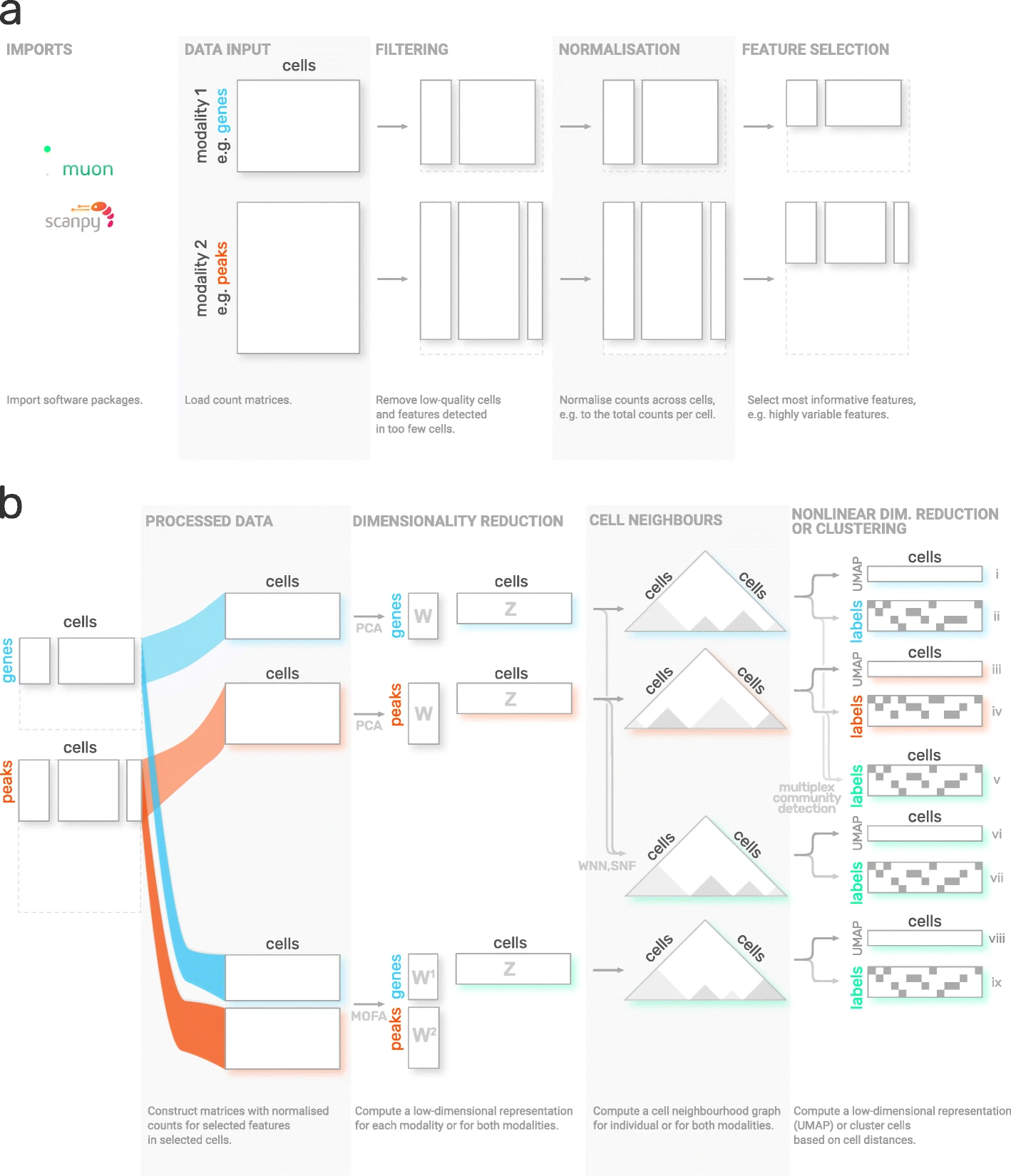
图 3:muon 概览。图片取自 Bredikhin et al., 2022。
安装
muon 可从 PyPI 获取,使用以下命令即可安装:
pip install muonAPI 概览
为介绍 muon,我们将查看一个多模态数据集中的 ATAC 数据。与 scanpy 章节类似,这里只快速演示并概览 muon,不会完整分析数据集,更不会给出最佳实践的多组学分析流程。请阅读相应章节,了解如何正确开展此类分析。
muon 从两个层面组织模块。首先,与 scanpy 类似,通用函数和多模态函数分别归入预处理(muon.pp),工具(muon.tl)和绘图(muon.pl)。其次,各类单模态工具位于 muon 中对应的模态模块下,并同样分为预处理、工具和绘图。例如,所有 ATAC 预处理函数都归入 muon.atac.pp。这也适用于 CITE-Seq 预处理功能(muon.prot.pp)。
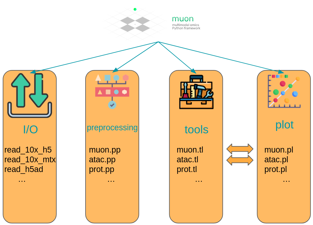
图 4:Muon 应用程序编程接口(application programming interface, API) 概览。模态特异的函数由相应命名的模块提供;用于联合分析多个模态的函数可直接通过 muon 模块调用。
Muon API 演示
本次演示使用一份公开的 10x Genomics Multiome 人 PBMC 数据集。
import muon as mu

mdata = ln.Artifact.get(
    key="introduction/advanced_data_structures_and_frameworks_muon.h5mu", is_latest=True
).load()

fragments = ln.Artifact.get(
    key="introduction/advanced_data_structures_and_frameworks_atac_fragments.tsv.gz",
    is_latest=True,
).cache()

fragments_tbi = ln.Artifact.get(
    key="introduction/advanced_data_structures_and_frameworks_atac_fragments.tsv.gz.tbi",
    is_latest=True,
).cache()

mdata作为第一步,我们将数据子集化到 ATAC 模态。
atac = mdata.mod["atac"]尽管现在处理的不是 RNA-seq 数据,仍可使用 scanpy 中同样适用于 ATAC 数据的部分预处理函数,因为两种模态具有相似的分布和质量问题。需要注意的是,在存放 ATAC-seq 数据的 AnnData 对象中,通常以峰(peak)代替基因作为特征。随后可使用 muon 的 ATAC 模块执行 ATAC 特有的预处理。
先进行一些质量控制(quality control, QC):过滤峰过少的细胞,以及只在过少细胞中检测到的峰。目前,我们会过滤掉未通过 QC 的细胞。
import scanpy as sc

sc.pp.calculate_qc_metrics(atac, percent_top=None, log1p=False, inplace=True)
sc.pl.violin(atac, ["total_counts", "n_genes_by_counts"], jitter=0.4, multi_panel=True)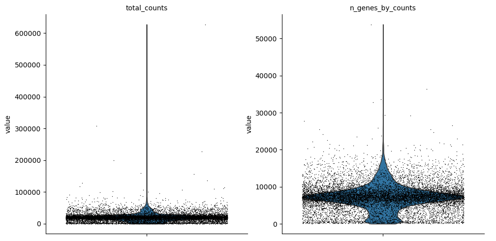
过滤掉未检测到可及性信号的峰。
mu.pp.filter_var(atac, "n_cells_by_counts", lambda x: x >= 10)
# This is analogous to
#   sc.pp.filter_genes(rna, min_cells=10)
# but does in-place filtering and avoids copying the object
我们也会过滤细胞。
mu.pp.filter_obs(atac, "n_genes_by_counts", lambda x: (x >= 2000) & (x <= 15000))
# This is analogous to
#   sc.pp.filter_cells(atac, max_genes=15000)
#   sc.pp.filter_cells(atac, min_genes=2000)
# but does in-place filtering avoiding copying the object

mu.pp.filter_obs(atac, "total_counts", lambda x: (x >= 4000) & (x <= 40000))
sc.pl.violin(atac, ["n_genes_by_counts", "total_counts"], jitter=0.4, multi_panel=True)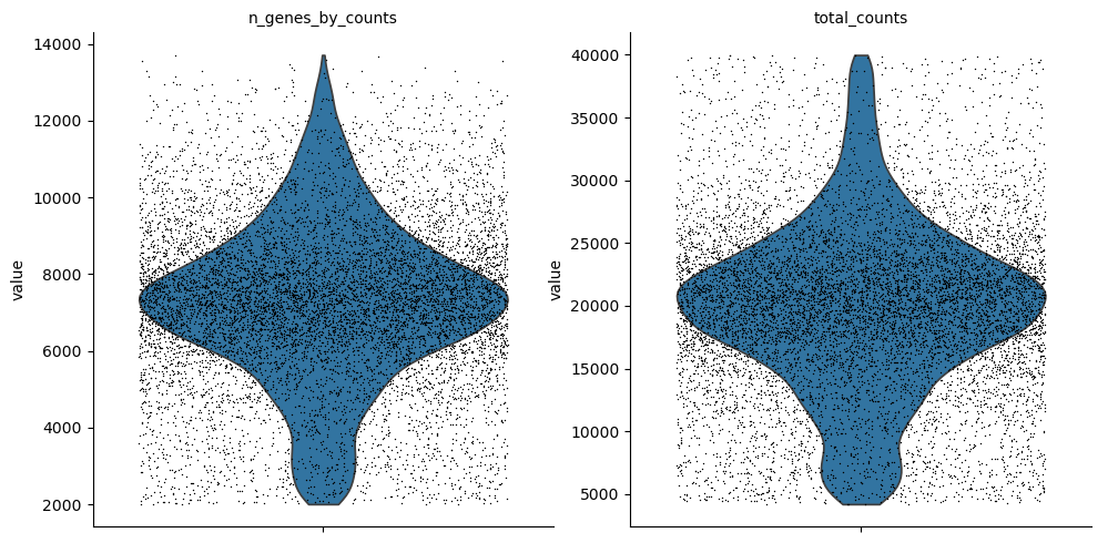
muon 还提供了直方图,让我们能从不同角度查看这些指标。
mu.pl.histogram(atac, ["n_genes_by_counts", "total_counts"])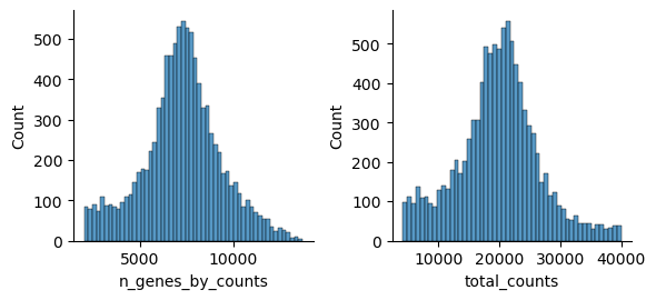
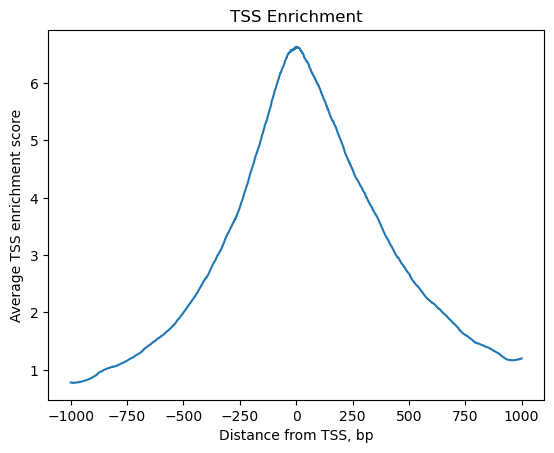
现在,我们已初步过滤掉了峰过少的细胞,以及只在过少细胞中被检测到的峰,接下来可以用 muon 开始进行 ATAC 特有的质量控制。muon 在相应模块中提供模态特有的预处理函数。我们导入 ATAC 模块,以使用 ATAC 特有的预处理函数。
from muon import atac as ac# Perform rudimentary quality control with muon's ATAC module
atac.obs["NS"] = 1
ac.tl.locate_fragments(mdata, fragments=str(fragments))
ac.tl.locate_fragments(atac, fragments=str(fragments))
ac.tl.nucleosome_signal(atac, n=1e6)
ac.tl.get_gene_annotation_from_rna(mdata["rna"]).head(3)
tss = ac.tl.tss_enrichment(mdata, n_tss=1000)
ac.pl.tss_enrichment(tss)Reading Fragments: 100%|██████████| 1000000/1000000 [00:03<00:00, 319214.51it/s]
Fetching Regions...: 100%|██████████| 1000/1000 [00:09<00:00, 106.91it/s]
# Save original counts, normalize data and select highly variable genes with scanpy
atac.layers["counts"] = atac.X
sc.pp.normalize_per_cell(atac, counts_per_cell_after=1e4)
sc.pp.log1p(atac)
sc.pp.highly_variable_genes(atac, min_mean=0.05, max_mean=1.5, min_disp=0.5)
atac.raw = atac
虽然 PCA 也常用于 ATAC 数据,但潜在语义索引(latent semantic indexing, LSI)是另一种常用方案,已在 muon 的 ATAC 模块中实现。
ac.tl.lsi(atac)
sc.pp.neighbors(atac, use_rep="X_lsi", n_neighbors=10, n_pcs=30)
sc.tl.leiden(atac, resolution=0.5)
sc.tl.umap(atac, spread=1.5, min_dist=0.5, random_state=20)
sc.pl.umap(atac, color=["leiden", "n_genes_by_counts"], legend_loc="on data")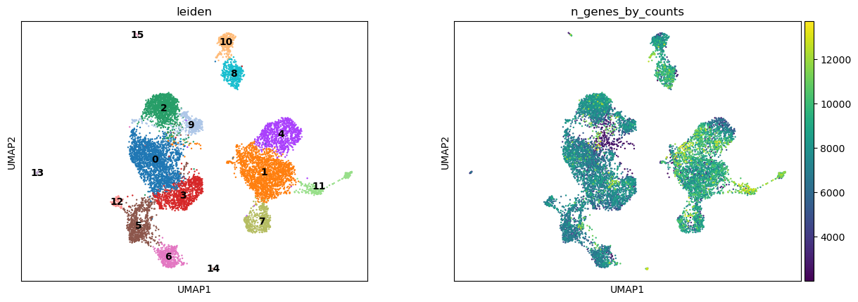
我们可以利用 muon 的 ATAC 模块,按某个基因所对应峰中的切割信号(cut value)为图形着色。
ac.pl.umap(atac, color=["KLF4"], average="peak_type")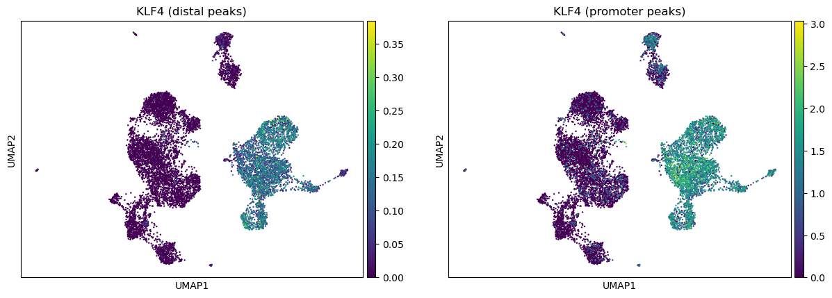
如需了解 muon 所有可用函数的更多信息,请阅读 muon API 参考 和 muon 教程。
使用 SpatialData 存储多模态与空间数据
空间组学(spatial omics)是指在保留分子信息(基因表达、染色质可及性、蛋白质)在组织内物理位置的同时对其进行测量的一类技术。传统的单细胞方法在组织解离过程中会丢失空间背景,而空间组学则同时保留单个细胞的分子谱和空间位置。由于这类数据集结合了图像、坐标和多种分子测量,因而体量庞大、结构复杂,需要专门的、具备空间感知能力的数据结构。SpatialData 统一了来自多种空间组学技术的原始数据和处理后数据 Marconato et al., 2025。它的五种基本元素(SpatialElement)按照 开放显微环境下一代文件格式(Open Microscopy Environment Next-Generation File Formats, OME-NGFF) 标准(一种用于生物成像数据的标准化格式)保存在 Zarr 存储中。
安装与导入
同样,使用 PyPI 或 Conda 来安装 SpatialData。
pip install spatialdata
conda install -c conda-forge spatialdata关键术语与数据模型
我们可以把 SpatialData 对象看作各种 Elements 的容器。Element 可以是 SpatialElement(Images,Labels,Points,Shapes)或 Table。下面是简要说明:
Images:苏木精–伊红染色(hematoxylin and eosin staining, H&E)图像Labels:像素级分割Points:带有基因信息的转录本位置、地标点Shapes:细胞/细胞核边界、亚细胞结构、解剖学注释和感兴趣区域(region of interest, ROI)Tables:用于注释SpatialElements的稀疏矩阵(sparse matrix)或稠密矩阵(dense matrix),或用于存储任意非空间元数据。它们不包含空间坐标。
我们可以把 SpatialElements 分为两大类:
Rasters:栅格数据(raster data)由像素组成,包括Images和LabelsVectors:矢量数据(vector data)由点和线组成。多边形也是矢量数据,因为它本质上是一组相连的点。Points和Shapes都属于这一类型。
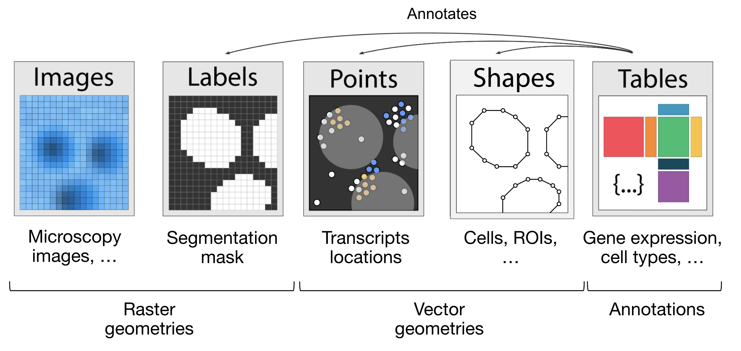
图 5:SpatialData 对象的各个元素。取自 。
import spatialdata as sd
import spatialdata_plot  # noqa: F401
让我们使用 lamindb 加载一个小鼠肝脏数据集。原始数据集见 此处。
sdata = ln.Artifact.get(
    key="introduction/advanced_data_structures_and_frameworks_spatialdata.zarr"
).load()
sdata
SpatialData object, with associated Zarr store: /Users/luisheinzlmeier/Library/Caches/lamindb/lamin-eu-central-1/VPwcjx3CDAa2/introduction/advanced_data_structures_and_frameworks_spatialdata.zarr
├── Images
│ └── 'raw_image': DataTree[cyx] (1, 6432, 6432), (1, 1608, 1608)
├── Labels
│ └── 'segmentation_mask': DataArray[yx] (6432, 6432)
├── Points
│ └── 'transcripts': DataFrame with shape: (<Delayed>, 3) (2D points)
├── Shapes
│ └── 'nucleus_boundaries': GeoDataFrame shape: (3375, 1) (2D shapes)
└── Tables
└── 'table': AnnData (3375, 99)
with coordinate systems:
▸ 'global', with elements:
raw_image (Images), segmentation_mask (Labels), transcripts (Points), nucleus_boundaries (Shapes)探索 Elements(SpatialData 对象)
让我们逐一探索每种元素类型及其表示方式:
图像:
xarray.DataArray或xarray.DataTree分别用于单尺度或多尺度图像的对象标签:
xarray.DataArray或xarray.DataTree对象,其中包含不同标签对应的整数编码点:
dask.DataFrame对象,包含点坐标(是pandas.DataFrame对象的惰性版本)形状:
geopandas.GeoDataFrame对象,其中包含多边形等几何对象表格:
anndata.AnnData对象,用于带注释的表格数据
sdata["raw_image"]输出
图像可以有多个尺度,这些尺度以降采样表示的形式存储在金字塔中,有助于更高效地可视化和分析。我们可以使用 get_pyramid_levels 函数来访问单个尺度,其中 0 是最高分辨率,1 按某个系数(通常为 2)进行降采样,2 再按另一个系数(通常为 2,相对于上一个尺度)进行降采样,依此类推。
本例图像有 2 个尺度(可查看 上方代码单元的输出分组)。让我们访问最高分辨率的图像。
sd.get_pyramid_levels(sdata["raw_image"], n=1)输出
要查看坐标轴和通道名称等图像属性,SpatialData 提供了一些辅助函数。更多辅助函数可在 API 页面中找到。坐标轴 x 和 y 表示图像的二维平面,而 c 对应图像内的不同通道(例如波长)。
sd.models.get_axes_names(sdata["raw_image"])('c', 'y', 'x')这里我们看到,我们的图像只有一个用于 4′,6-二脒基-2-苯基吲哚(4′,6-diamidino-2-phenylindole, DAPI) 染色的通道(用于突出显示细胞核)。
sd.models.get_channel_names(sdata["raw_image"])[0]下面使用 spatialdata-plot 来显示图像(用于细胞核的 DAPI 染色)。
sdata.pl.render_images("raw_image", cmap="gray").pl.show()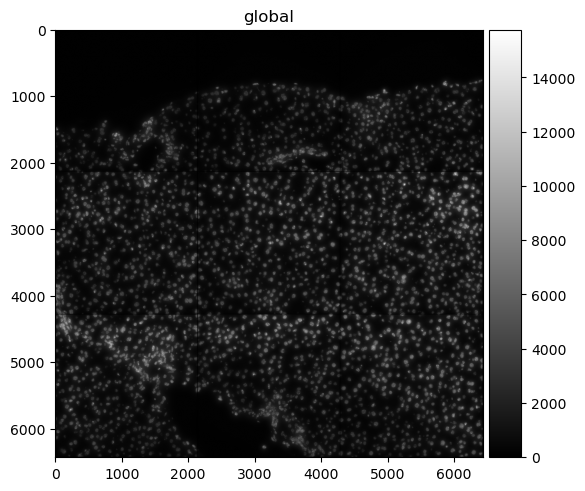
点
点表示为 dask.DataFrame 对象,其中包含点坐标(它是 pandas.DataFrame 对象的惰性版本)。惰性加载(lazy loading)DataFrame 可以减少内存用量,因为信息只在需要时才从数据文件中读取,而不会一次性全部载入。对于测量单分子的空间转录组数据集,坐标存储在列 x 和 y(可选地还包括 z 用于三维数据),并另有一列用于注释基因身份。
sdata["transcripts"]我们可以轻松地将 dask.DataFrame 转换为一个 pandas.DataFrame,具体可调用 .compute(),以便更轻松地操作。请注意,这会将整个对象载入内存。如果数据很大,可以直接使用 dask 的 API 来操作该 DataFrame。
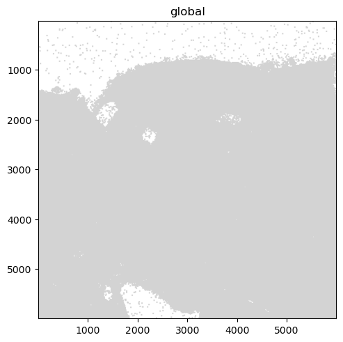
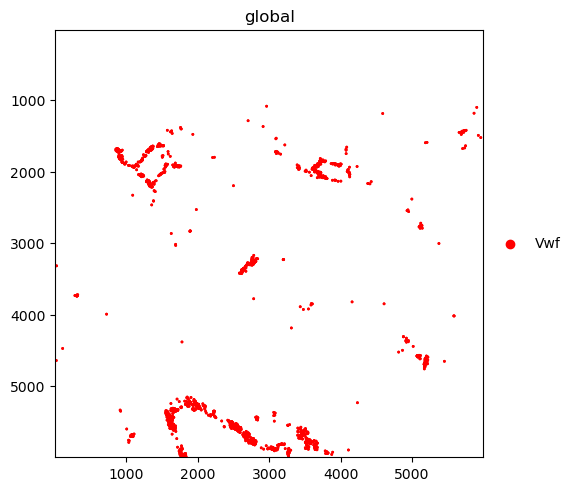
sdata["transcripts"].compute()可视化这些点时,绘图后端会自动切换:从 matplotlib 到 datashader。这确保了在点数很大时仍能高效渲染。如下所示,绘制转录本的子集(例如特定基因)会更有用。
我们进一步绘制按基因着色的转录本。其中的 groups 参数可用于绘制一部分基因的转录本。
sdata.pl.render_points("transcripts").pl.show()
sdata.pl.render_points(
    "transcripts", color="gene", groups="Vwf", palette="red", table_name="table"
).pl.show()
INFO Using 'datashader' backend with 'None' as reduction method to speed up plotting. Depending on the
reduction method, the value range of the plot might change. Set method to 'matplotlib' do disable this
behaviour.
WARNING No table name provided, using 'table' as fallback for color mapping.
形状
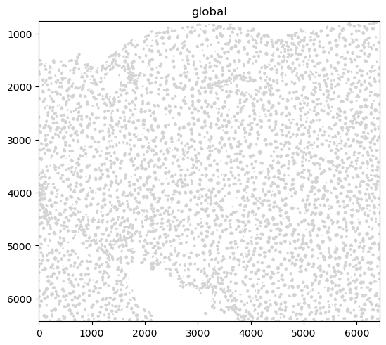
形状表示为 geopandas.GeoDataFrame,即包含多边形等几何对象的对象。关于如何使用 geopandas.GeoDataFrame 对象,请参阅 geopandas 文档。
sdata["nucleus_boundaries"]sdata.pl.render_shapes("nucleus_boundaries").pl.show()INFO Converted 1 Polygon(s) with holes to MultiPolygon(s) for correct rendering.
表格
带注释的矩阵表示为 anndata.AnnData 对象。导入后的数据集通常会在 sdata['table'] 处放置一个用于计数/丰度矩阵的表格。这样便可使用 Scanpy、scVI 等工具进行下游分析。
对于不同空间技术,这里量化的是:
转录组学:转录本计数;
空间蛋白质组学:标记物丰度;
基于载玻片的测定:点位/网格丰度(参见空间组学章节)。
sdata["table"]输出
AnnData object with n_obs × n_vars = 3375 × 99
    obs: 'cell_ID', 'fov_labels', 'annotation'
    uns: 'spatialdata_attrs', 'annotation_colors'
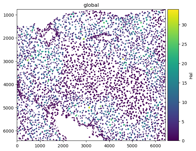
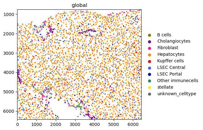
obsm: 'spatial'下面演示如何在细胞上绘制数值信息(HAL 基因表达),并绘制分类信息(细胞类型)。
sdata.pl.render_shapes("nucleus_boundaries", color="Hal").pl.show()
sdata.pl.render_shapes("nucleus_boundaries", color="annotation").pl.show()
INFO Converted 1 Polygon(s) with holes to MultiPolygon(s) for correct rendering.
INFO Successfully extracted 10 colors from 'annotation_colors' in table 'table'.
INFO Converted 1 Polygon(s) with holes to MultiPolygon(s) for correct rendering.
使用 Squidpy 进行空间组学数据分析
Squidpy 是一个用于分析和可视化空间组学数据的框架。它的发表大约比 SpatialData 早两年 Marconato et al., 2025Palla et al., 2022。这也是为什么 Squidpy 最初构建在 Scanpy 和 AnnData 之上。由于 scverse 生态系统将逐步让 Squidpy 在内部改用 SpatialData,因此这里只简要介绍 Squidpy 如何使用空间数据。更多后续变化和教程,请查阅以下文档:SpatialData 和 Squidpy。
API 概览
Squidpy 的 API 允许您分析和可视化空间分子数据。图(gr)处理空间关系和相互作用,图像(im)负责处理并分割组织图像,工具(tl)提供空间分析,绘图(pl)可视化数据和结果。读取(read)和数据集(datasets)支持跨各种技术导入数据和示例数据集。
安装并导入软件包
Squidpy 可在 PyPI 和 Conda 上获取,可使用以下任一命令安装。
pip install squidpy
conda install -c conda-forge squidpy
SpatialData 集成
让我们从导入 Squidpy 开始。
import squidpy as sq可以用以下工具加载 Xenium 数据集:lamindb。
sdata = ln.Artifact.get(
    key="introduction/advanced_data_structures_and_frameworks_squidpy.zarr"
).load()
sdata
SpatialData object, with associated Zarr store: /Users/luisheinzlmeier/Library/Caches/lamindb/lamin-eu-central-1/VPwcjx3CDAa2/introduction/advanced_data_structures_and_frameworks_squidpy.zarr
├── Images
│ ├── 'morphology_focus': DataTree[cyx] (1, 25778, 35416), (1, 12889, 17708), (1, 6444, 8854), (1, 3222, 4427), (1, 1611, 2213)
│ └── 'morphology_mip': DataTree[cyx] (1, 25778, 35416), (1, 12889, 17708), (1, 6444, 8854), (1, 3222, 4427), (1, 1611, 2213)
├── Points
│ └── 'transcripts': DataFrame with shape: (<Delayed>, 8) (3D points)
├── Shapes
│ ├── 'cell_boundaries': GeoDataFrame shape: (167780, 1) (2D shapes)
│ └── 'cell_circles': GeoDataFrame shape: (167780, 2) (2D shapes)
└── Tables
└── 'table': AnnData (167780, 313)
with coordinate systems:
▸ 'global', with elements:
morphology_focus (Images), morphology_mip (Images), transcripts (Points), cell_boundaries (Shapes), cell_circles (Shapes)Squidpy 演示
下面计算 Xenium 数据集空间坐标的近邻图(nearest-neighbor graph)。
sq.gr.spatial_neighbors(sdata["table"])之后,可以根据基因表达谱对细胞进行聚类(clustering)。
%%time
sc.pp.pca(sdata["table"])
sc.pp.neighbors(sdata["table"])
sc.tl.leiden(sdata["table"])
CPU times: user 2min 6s, sys: 3.94 s, total: 2min 10s
Wall time: 2min 10s
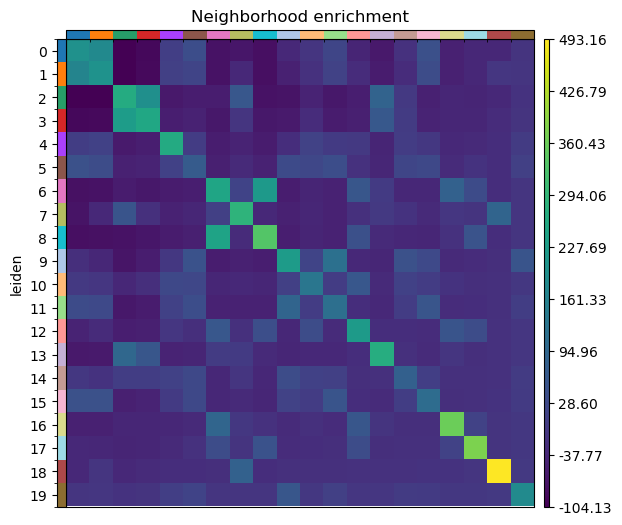
然后在 Squidpy 中运行邻域富集(neighborhood enrichment)分析。
sq.gr.nhood_enrichment(sdata["table"], cluster_key="leiden")
sq.pl.nhood_enrichment(sdata["table"], cluster_key="leiden", figsize=(5, 5))
100%|██████████| 1000/1000 [00:44<00:00, 22.28/s]
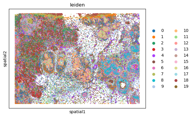
最后,我们既可以用 Squidpy,也可以用 SpatialData 中新的绘图函数,在空间坐标中将结果可视化。
%%time
sq.pl.spatial_scatter(sdata["table"], shape=None, color="leiden")
WARNING: Please specify a valid `library_id` or set it permanently in `adata.uns['spatial']`
CPU times: user 112 ms, sys: 6.02 ms, total: 118 ms
Wall time: 117 ms
选择题
- Virshup, I., Rybakov, S., Theis, F. J., Angerer, P., & Wolf, F. A. (2021). anndata: Annotated data. bioRxiv. 10.1101/2021.12.16.473007
- Wolf, F. A., Angerer, P., & Theis, F. J. (2018). SCANPY: large-scale single-cell gene expression data analysis. Genome Biology, 19(1), 15. 10.1186/s13059-017-1382-0
- Bredikhin, D., Kats, I., & Stegle, O. (2022). MUON: multimodal omics analysis framework. Genome Biology, 23(1), 42. 10.1186/s13059-021-02577-8
- Palla, G., Spitzer, H., Klein, M., Fischer, D., Schaar, A. C., Kuemmerle, L. B., Rybakov, S., Ibarra, I. L., Holmberg, O., Virshup, I., Lotfollahi, M., Richter, S., & Theis, F. J. (2022). Squidpy: a scalable framework for spatial omics analysis. Nature Methods, 19(2), 171–178. 10.1038/s41592-021-01358-2
- Marconato, L., Palla, G., Yamauchi, K. A., Virshup, I., Heidari, E., Treis, T., Vierdag, W.-M., Toth, M., Stockhaus, S., Shrestha, R. B., Rombaut, B., Pollaris, L., Lehner, L., Vöhringer, H., Kats, I., Saeys, Y., Saka, S. K., Huber, W., Gerstung, M., … Stegle, O. (2025). SpatialData: an open and universal data framework for spatial omics. Nature Methods, 22(1), 58–62. 10.1038/s41592-024-02212-x