🧠 关键要点
结合两种互补方法进行双细胞(Doublet)评分:一种比较模拟 Doublet 的计数(Count)分布,另一种统计被两个以上独立片段覆盖的基因组位点。后者依赖足够的测序深度,原文建议每个细胞超过约 10,000–15,000 个读段(Read)。
结合片段总数、特征(feature)数,以及单细胞转座酶可及染色质测序(single-cell assay for transposase-accessible chromatin using sequencing, scATAC-seq)特有的转录起始位点(Transcription Start Site, TSS)富集分数、核小体信号(nucleosome signal)进行质量控制(Quality Control, QC)。检查各项指标的极端值,并重点识别片段数少且 TSS 富集低的细胞条形码(cell barcode, CB)。阈值应结合样本分布确定。
根据细胞总数和研究目标过滤 feature。不关注稀有状态时,可考虑仅保留至少在 1% 细胞中检测到的 feature;研究稀有群体时,应结合其预期丰度和检测概率,选择合适的最小检测细胞数。
⚙️ 环境设置
安装 conda:
在创建环境之前,请确保 conda 已安装在你的系统中。
保存 yml 内容:
将 yml 选项卡中的内容保存为文件
environment.yml。
创建环境:
打开终端或命令提示符。
运行以下命令:
conda env create -f environment.yml
激活环境:
创建好环境后,使用以下命令激活它:
conda activate <environment_name>请将
<environment_name>替换为environment.yml文件中指定的环境名称。该名称在 yml 文件中如下所示:name: <environment_name>
验证安装:
通过运行以下命令,检查环境是否创建成功:
conda env list
🗄️ 获取数据和笔记本
本书使用 lamindb 存储、共享和加载数据集与笔记本,使用的实例为 theislab/sc-best-practices 实例。感谢以下机构提供免费托管:Lamin Labs。
安装 lamindb
安装 lamindb Python 软件包:
pip install lamindb可选择创建 Lamin 账户
请按照 相关说明注册并登录
验证你的设置
运行
lamin connect命令:
import lamindb as ln

ln.Artifact.connect("theislab/sc-best-practices").df()
你现在应该能看到最多 100 个已存储的数据集。
访问数据集(Artifact)
在以下页面搜索数据集:Artifacts 页面
加载一个 Artifact 及其对应的对象:
import lamindb as ln
af = ln.Artifact.connect("theislab/sc-best-practices").get(key="key_of_dataset", is_latest=True)
obj = af.load()
对象已加载到内存,可用于分析。要获取相应版本,可调整
lamindb.Artifact.connect("theislab/sc-best-practices").get("SOMEIDXXXX")中的版本标识。访问笔记本(Transform)
在以下页面搜索笔记本:Transforms 页面
加载笔记本:
lamin load <notebook url>该命令会将笔记本下载到当前工作目录。与
Artifacts类似,你也可以调整后缀 ID 来获取旧版本。
研究动机
去除低质量细胞是单细胞分析的重要环节,否则下游结果可能受到干扰。单细胞转座酶可及染色质测序(single-cell assay for transposase-accessible chromatin using sequencing, scATAC-seq)通常只能在每个细胞中检测到约 1%–10% 的开放区域,数据比单细胞 RNA 测序(Single-Cell RNA Sequencing, scRNA-seq)更稀疏 Chen et al., 2019。测序深度不足或信噪比(signal-to-noise ratio, SNR)较低时,细胞提供的有效信息可能很少。另一项挑战是识别多细胞混合体(multiplet),即两个或更多细胞被共同测量。本章介绍 scATAC-seq 的质量控制(Quality Control, QC)指标及双细胞(Doublet)检测方法。
数据集
本章使用为 NeurIPS 2021 单细胞数据整合挑战赛生成的 10x Multiome 数据集演示 scATAC-seq 处理 Luecken et al., 2021。该数据集包含多个样本,联合分析前需统一特征(feature)的定义并考虑数据整合,后续章节将进一步讨论。质量评估则应尽量逐样本开展,以免样本间差异干扰判断。因此,本笔记本仅对其中一个样本进行预处理。
分析从 cellranger-arc 的输出开始。这是 10x 为 Multiome 测定(Assay)提供的比对、峰识别(peak calling)及初步 QC 软件,默认输出包含单细胞核 RNA 测序(Single-Nucleus RNA Sequencing, snRNA-seq)与 scATAC-seq 数据。RNA 数据预处理已在前文介绍,这里只处理染色质可及性(chromatin accessibility)数据;相同步骤也适用于单模态 scATAC-seq。
首先读取 filtered_feature_bc_matrix.h5 文件,其中包含细胞 × 峰的计数矩阵(Count matrix)。读取时,muon 还会自动查找同一目录下的片段文件和峰注释文件。
先导入所需的 Python 包。
# Single-cell packages
import anndata2ri
import matplotlib.pyplot as plt
import muon as mu
import numpy as np

# General helpful packages for data analysis and visualization
import pandas as pd
import scanpy as sc
import seaborn as sns
from muon import atac as ac  # the module containing function for scATAC data processing

# Packages enabling to run R code
from rpy2.robjects import pandas2ri

pandas2ri.activate()  # Automatically convert rpy2 outputs to pandas DataFrames
anndata2ri.activate()
%load_ext rpy2.ipython


# Setting figure parameters
sc.settings.verbosity = 0
sns.set(rc={"figure.figsize": (4, 3.5), "figure.dpi": 100})
sns.set_style("whitegrid")
The rpy2.ipython extension is already loaded. To reload it, use:
%reload_ext rpy2.ipython
mdata = mu.read_10x_h5("cellranger_out/filtered_feature_bc_matrix.h5")输出
/Users/christopher.lance/mambaforge/envs/scatac_pp/lib/python3.9/site-packages/anndata/_core/anndata.py:1830: UserWarning: Variable names are not unique. To make them unique, call `.var_names_make_unique`.
  utils.warn_names_duplicates("var")
Added `interval` annotation for features from resources/cellranger_out/filtered_feature_bc_matrix.h5
/Users/christopher.lance/mambaforge/envs/scatac_pp/lib/python3.9/site-packages/anndata/_core/anndata.py:1830: UserWarning: Variable names are not unique. To make them unique, call `.var_names_make_unique`.
  utils.warn_names_duplicates("var")
/Users/christopher.lance/mambaforge/envs/scatac_pp/lib/python3.9/site-packages/mudata/_core/mudata.py:446: UserWarning: var_names are not unique. To make them unique, call `.var_names_make_unique`.
  warnings.warn(
Added peak annotation from resources/cellranger_out/atac_peak_annotation.tsv to .uns['atac']['peak_annotation']
Added gene names to peak annotation in .uns['atac']['peak_annotation']
Located fragments file: resources/cellranger_out/atac_fragments.tsv.gz
警告提示峰标识符存在重复。为避免影响下游分析,使用 .var_names_make_unique() 方法将名称变为唯一值。
mdata.var_names_make_unique()查看刚创建的 MuData 对象。
mdataRNA 和 ATAC 分别存储在两个 AnnData 对象中,共载入 16,934 个细胞;RNA 模态包含 36,601 个基因,ATAC 模态包含 154,027 个峰。ATAC 的非结构化数据槽 atac.uns 还保存了峰注释与片段文件路径,均由以下包自动定位:muon。
查看 atac.uns 中的峰注释和片段文件路径。
mdata.mod["atac"].unsOverloadedDict, wrapping:
OrderedDict([('atac', {'peak_annotation': peak distance peak_type
gene_name
MIR1302-2HG chr1:9763-10648 -18906 distal
AL627309.1 chr1:115270-116168 4764 distal
AL627309.5 chr1:181107-181768 -7246 distal
AL627309.5 chr1:183973-184845 -10112 distal
AL627309.5 chr1:191237-192111 -17376 distal
... ... ... ...
AC213203.2 KI270713.1:21361-22256 10272 distal
AC213203.2 KI270713.1:29645-30508 2020 distal
AC213203.2 KI270713.1:32401-33088 0 promoter
AC213203.1 KI270713.1:34369-35136 -271 promoter
AC213203.1 KI270713.1:36970-37884 1564 distal
[196633 rows x 3 columns]}), ('files', {'fragments': 'resources/cellranger_out/atac_fragments.tsv.gz'})])
With overloaded keys:
['neighbors'].峰注释表提供了峰与基因可能相关的初步线索。不过,这里主要依据峰到最近基因的距离进行注释,不能据此认定该峰调控相应基因。
提取 ATAC 模态对应的 Anndata 对象,用于后续处理:
atac = mdata.mod["atac"]Doublet 检测
scATAC-seq 的稀疏性更高,不宜直接照搬 scRNA-seq 的 Doublet 检测流程。这里采用两种互补的评分方法,后续结合细胞聚类(clustering)识别疑似 Doublet 群体。两种方法均可通过 R 包 scDblFinder 使用 Germain et al., 2021;以下步骤参考了 这份教程。
方法 1:根据模拟 Doublet 评分。scDblFinder 通过生成模拟 Doublet 计算分数(参见 Doublet 检测)。生成模拟数据前,先聚合高度相关的 feature,以降低稀疏性和维度。与 scRNA-seq 中的类似方法一样,这一策略主要识别由不同细胞类型组成的异型 Doublet(heterotypic doublet)。
方法 2:使用 AMULET 根据覆盖度评分。 Thibodeau et al., 2021 其依据是二倍体常染色体位点通常只有两份 DNA 模板。AMULET 统计被两个以上独立片段覆盖的位点数(见下图);这类位点异常增多时,提示可能存在 Doublet。重复未充分去除、测序或比对错误、重复序列等也会造成少量异常覆盖,因此不能把单个位点的异常直接视为 Doublet。该方法需要足够的测序深度,原文建议每个细胞超过约 10,000–15,000 个读段(Read);它既可识别异型 Doublet,也有助于发现同一类型细胞组成的同型 Doublet(homotypic doublet)。
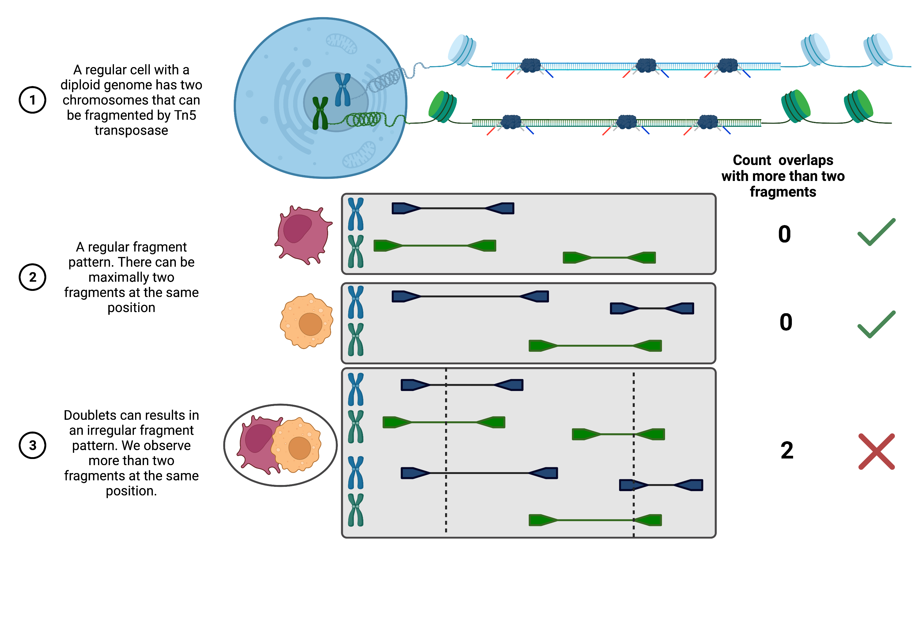
图 1:AMULET 方法概述。
运行 Doublet 检测前,先检查 R 的包库路径是否指向已配置的环境。
%%R
.libPaths()
[1] "/Users/christopher.lance/mambaforge/envs/scatac_pp/lib/R/library"
加载 scDblFinder 和 SingleCellExperiment 包。
%%R
suppressPackageStartupMessages(library(scDblFinder))
suppressPackageStartupMessages(library(SingleCellExperiment))
基于 Count 分布的 Doublet 评分
Doublet 评分可能耗时较长,先指定输出目录和样本标识,便于保存结果。
# Set output paths
save_path_dir = "output/doublet_scores/"
sample_ident = "s4d8"
为把数据传入 R 的 SingleCellExperiment 对象,先转置矩阵(.T),再将 atac.X 中的稀疏矩阵(sparse matrix)转成稠密数组(.A);同时单独保存细胞条形码(cell barcode, CB)列表。稠密化会增加内存开销,应根据矩阵大小评估可用内存。
barcodes = list(atac.obs_names)
data_mat = atac.X.T.A
这里的 scDblFinder 函数接收 SingleCellExperiment 对象;我们用 data_mat 构造该对象。模拟 Doublet 时,可通过 clusters 参数选择基于聚类或随机配对细胞。外周血单个核细胞(Peripheral Blood Mononuclear Cells, PBMCs)等群体边界清晰的数据适合基于聚类;连续轨迹数据通常更适合随机配对。可以提供逐细胞的簇标签向量、指定 SingleCellExperiment 中存放标签的元数据列,或设为 TRUE 以自动聚类。若要随机配对而不使用聚类,则设为 clusters=FALSE 或 clusters=NULL。直接使用全部峰或基因组窗口的计算成本较高,作者建议将相关 feature 聚合为较少的 聚合特征(meta-feature)Germain et al., 2021。设置 aggregateFeatures=TRUE 即可启用聚合,将峰或窗口的 Count 汇总为 nfeatures 个 meta-feature;本例取 25。随后通过 processing="normFeatures" 对聚合后的 feature 归一化(normalization),再计算 Doublet 分数。
%R -i data_mat -o dbl_score sce <- scDblFinder(SingleCellExperiment(list(counts=data_mat)), \
                                               clusters=TRUE, aggregateFeatures=TRUE, nfeatures=25, \
                                               processing="normFeatures"); dbl_score <- sce$scDblFinder.score
输出
R[write to console]: dimnames(.) <- NULL translated to
dimnames(.) <- list(NULL,NULL)

R[write to console]: Aggregating features...

R[write to console]: Clustering cells...

R[write to console]: Warnung in (function (A, nv = 5, nu = nv, maxit = 1000, work = nv + 7, reorth = TRUE,
R[write to console]:

R[write to console]:  You're computing too large a percentage of total singular values, use a standard svd instead.

R[write to console]: 8 clusters

R[write to console]: Creating ~13548 artificial doublets...

R[write to console]: Dimensional reduction

R[write to console]: Evaluating kNN...

R[write to console]: Training model...

R[write to console]: iter=0, 2617 cells excluded from training.

R[write to console]: iter=1, 2725 cells excluded from training.

R[write to console]: iter=2, 2756 cells excluded from training.

R[write to console]: Threshold found:0.466

R[write to console]: 3038 (17.9%) doublets called

/Users/christopher.lance/mambaforge/envs/scatac_pp/lib/python3.9/site-packages/anndata2ri/r2py.py:106: FutureWarning: X.dtype being converted to np.float32 from float64. In the next version of anndata (0.9) conversion will not be automatic. Pass dtype explicitly to avoid this warning. Pass `AnnData(X, dtype=X.dtype, ...)` to get the future behavour.
  return AnnData(exprs, obs, var, uns, obsm or None, layers=layers)
array([0.02819141, 0.00082514, 0.06341238, ..., 0.15534039, 0.02116382,
       0.12427134])
输出提示约 18% 的细胞被判为 Doublet。这个比例较高,但作者认为,与本样本的细胞加载量及分离细胞核容易粘连的特点相符。它仍是模型判断,应结合后续诊断核对。
计算完成后,创建 pandas.DataFrame,保存所有 Barcode 的分数并写入文件。
scDbl_result = pd.DataFrame({"barcodes": barcodes, "scDblFinder_score": dbl_score})
scDbl_result.to_csv(save_path_dir + "/scDblFinder_scores_" + sample_ident + ".csv")scDbl_result.head()为将分数写入 ATAC 的 AnnData 对象,先把 Barcode 设为数据框索引,以便按细胞名称与观测表对齐。原文将该表泛称为 adata.obs。
scDbl_result = scDbl_result.set_index("barcodes")然后添加分数列;下方代码实际写入 atac.obs,原文泛称 adata.obs。
atac.obs["scDblFinder_score"] = scDbl_result["scDblFinder_score"]基于覆盖度的 Doublet 评分
AMULET 根据覆盖度大于 2 的基因组位点数判断异常。这一模型基于二倍体常染色体,因此按 Thibodeau et al., 2021 的建议排除线粒体基因组和性染色体;线粒体 DNA 在一个细胞中可有多份拷贝。此外,还需屏蔽散在重复元件、卫星重复等区域。我们使用随 AMULET 论文提供的 .bed 文件,该文件可从以下平台下载:Zenodo。用 R 包 rtracklayer 读入后,可直接得到 GRanges 对象。本例约有 16,000 个细胞,作者在个人电脑上运行约需 4 小时;实际耗时取决于硬件和数据。重复区域的 .bed 文件及 AMULET 输出也可从 figshare 获取。
%%R

# Set up a GRanges objects of repeat elements, mitochondrial genes and sex chromosomes we want to exclude
suppressPackageStartupMessages(library(GenomicRanges))
suppressPackageStartupMessages(library(rtracklayer))

repeats =  import('resources/blacklist_repeats_segdups_rmsk_hg38.bed')
otherChroms <- GRanges(c("chrM","chrX","chrY","MT"),IRanges(1L,width=10^8)) # check which chromosome notation you are using c("M", "X", "Y", "MT")
toExclude <- suppressWarnings(c(repeats, otherChroms))
再获取片段文件的路径。
frag_path = atac.uns["files"]["fragments"]
frag_path'resources/cellranger_out/atac_fragments.tsv.gz'现在运行 AMULET。通过 -i 和 -o 分别声明从 Python 传入的对象和要返回 Python 的结果;这两个参数跟在 %R 魔术命令(magic)后。toExclude 已在 R 环境中创建,可直接由 amulet 使用。若可用内存充足,可考虑 fullInMemory=TRUE 选项以缩短运行时间。
# Run AMULET
%R -i frag_path -o amulet_result amulet_result <- amulet(frag_path, regionsToExclude=toExclude)

# Save output
amulet_result.to_csv(save_path_dir + "/AMULET_scores_" + sample_ident + ".csv")
输出
R[write to console]: 18:01:17 - Reading Tabix-indexed fragment file and computing overlaps
chr1, chr10, chr11, chr12, chr13, chr14, chr15, chr16, chr17, chr18, chr19, chr2, chr20, chr21, chr22, chr3, chr4, chr5, chr6, chr7, chr8, chr9, chrX, chrY, KI270728.1, KI270727.1, GL000009.2, GL000194.1, GL000205.2, GL000195.1, GL000219.1, KI270734.1, GL000213.1, GL000218.1, KI270731.1, KI270721.1, KI270726.1, KI270711.1, KI270713.1,
R[write to console]: 22:20:44 - Merging
查看 AMULET 的输出。
amulet_result.head()AMULET 为每个 Barcode 返回片段数、被两个以上片段覆盖的位点数,以及检验“该观测为单个细胞(singlet)”零假设(null hypothesis)的 p 值(p-value)和多重检验(multiple testing)校正后的 q 值。q-value 越低,反对 singlet 假设的证据越强,但它不是 Doublet 概率。可以使用显著性阈值分类;本例先保留分数,之后通过可视化综合识别疑似 Doublet 群体。
把这些结果也写入 atac 对象,并将 q 值转换为 −log10(q),便于绘图。
atac.obs["AMULET_pVal"] = amulet_result["p.value"]
atac.obs["AMULET_qVal"] = amulet_result["q.value"]
# Transform q-values for nicer plotting
atac.obs["AMULET_negLog10qVal"] = -1 * np.log10(amulet_result["q.value"])/Users/christopher.lance/mambaforge/envs/scatac_pp/lib/python3.9/site-packages/pandas/core/arraylike.py:402: RuntimeWarning: divide by zero encountered in log10
result = getattr(ufunc, method)(*inputs, **kwargs)
比较两种方法的评分结果。
atac.obs.plot(x="scDblFinder_score", y="AMULET_negLog10qVal", kind="scatter")

plt.title("Association of doublet scores")
plt.show()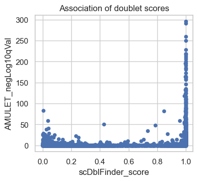
散点图横轴为 scDblFinder 分数,纵轴为 AMULET 的 −log10(q),每个点代表一个 Barcode。右上方表示两种方法都提供较强的 Doublet 证据;左下方表示两者均未显示明显异常。右下方主要由 scDblFinder 提示异常;左上方的少数点主要由 AMULET 提示异常,可能包含 scDblFinder 较难发现的同型 Doublet。这些分数并非已经确定的细胞身份,后续还需结合聚类判断。
计算 QC 指标
以下指标常用于 scATAC-seq 处理流程,帮助识别低质量细胞:
total_fragment_counts:每个细胞的总 Count,可反映测序深度,类似 scRNA-seq 的总 Count。下方代码从峰矩阵求和得到此列,其含义受矩阵计数口径限制,并非片段文件中的全部唯一片段数。
tss_enrichment:转录起始位点(Transcription Start Site, TSS)富集分数,衡量 TSS 中心附近信号相对于两侧背景的富集程度,可用于评估信噪比。
n_features_per_cell:每个细胞中 Count 非零的峰数,类似 scRNA-seq 中检测到的基因数。
nucleosome_signal:核小体信号(nucleosome signal),即单核小体片段数与无核小体片段数之比,用于评估文库质量,详见下文。该比值通常越高越需要关注,不能按“越高越好”的信噪比理解。
还可考虑以下指标:
reads_in_peaks_frac: 峰内 Read 比例(Fraction of Reads in Peaks, FRiP),通常以峰内 Read 数除以总 Read 数;使用片段计数的实现则按片段统计。它反映信号相对于背景的富集,分母并非仅峰外部分。
blacklist_fraction: 落在 ENCODE 黑名单区域内的片段比例。这些区域容易产生技术伪影。根据 scATAC-seq 基准研究 Chen et al., 2019 及作者的分析经验,这一问题在所考察的单细胞数据中通常不严重,但仍应结合数据检查。
除逐细胞 QC 外,还应评估样本整体质量,例如比较各样本检测到的细胞数和 QC 指标分布。按样本分组的小提琴图有助于发现样本间差异。
总 Count 与 feature 数
先用 Scanpy 的 calculate_qc_metrics 函数计算每个细胞在峰矩阵中的总 Count 和非零 feature 数。由于输出列名沿用 RNA-seq 术语,这里将 total_counts 重命名为 total_fragment_counts 和 n_genes_by_counts 重命名为 n_features_per_cell。为便于绘图,还对 total_fragment_counts 取以 10 为底的对数。
# Calculate general qc metrics using scanpy
sc.pp.calculate_qc_metrics(atac, percent_top=None, log1p=False, inplace=True)

# Rename columns
atac.obs.rename(
    columns={
        "n_genes_by_counts": "n_features_per_cell",
        "total_counts": "total_fragment_counts",
    },
    inplace=True,
)

# log-transform total counts and add as column
atac.obs["log_total_fragment_counts"] = np.log10(atac.obs["total_fragment_counts"])核小体信号
接下来计算 scATAC-seq 特有的核小体信号和 TSS 富集分数。
计算核小体信号时,参数 n 限制整次计算读取的片段总数,并非每个细胞各读取这么多。下方设置为 10e3 × 细胞数,也就是 10,000 × 细胞数。以 muon 0.1.4 的实现为例,这与其默认值 1e4 × 细胞数相同,并非原文所称的缩小十倍。正式分析应核对所用版本的默认值,并在计算成本与估计稳定性之间取舍。
# Calculate the nucleosome signal across cells
# set n=10e3*atac.n_obs for rough estimate but faster run time
ac.tl.nucleosome_signal(atac, n=10e3 * atac.n_obs)
Reading Fragments: 100%|██████████████████████████████████████████████████████████████████████████████████████████████████████████████████████████████████| 169340000/169340000 [08:54<00:00, 317005.72it/s]
先查看核小体信号的总体分布。
sns.histplot(atac.obs, x="nucleosome_signal")
plt.title("Distribution of the nucleome signal")
plt.show()

# Alternatively as a violin plot (uncomment to plot)
# sc.pl.violin(atac, "nucleosome_signal")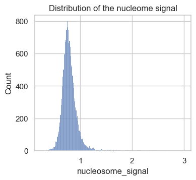
本数据集的核小体信号约在 0–3 之间。以往项目常在 2–4 之间选择上限,但这只是经验范围。本例用 2 将细胞分为两组,在 atac.obs 中保存标签,以比较高、低核小体信号对应的片段长度分布。
# Add group labels for above and below the nucleosome signal threshold
nuc_signal_threshold = 2
atac.obs["nuc_signal_filter"] = [
    "NS_FAIL" if ns > nuc_signal_threshold else "NS_PASS"
    for ns in atac.obs["nucleosome_signal"]
]

# Print number cells not passing nucleosome signal threshold
atac.obs["nuc_signal_filter"].value_counts()
NS_PASS 16877
NS_FAIL 57
Name: nuc_signal_filter, dtype: int64atac.obs["nuc_signal_filter"] # = atac.obs["nuc_signal_filter"].astype('category')AAACAGCCAAGCTTAT-1 NS_PASS
AAACAGCCATAGCTTG-1 NS_PASS
AAACAGCCATGAAATG-1 NS_PASS
AAACAGCCATGTTTGG-1 NS_PASS
AAACATGCAACGTGCT-1 NS_PASS
...
TTTGTTGGTGGCTTCC-1 NS_PASS
TTTGTTGGTTCTTTAG-1 NS_PASS
TTTGTTGGTTGGCCGA-1 NS_PASS
TTTGTTGGTTTACTTG-1 NS_PASS
TTTGTTGGTTTGTGGA-1 NS_PASS
Name: nuc_signal_filter, Length: 16934, dtype: object本样本中,核小体信号高于 2 的 Barcode 只有 57 个。
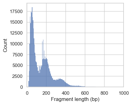
分别绘制两组细胞的片段长度分布。为减少计算量,仅考察 1 号染色体上的指定区域,设置为 region="chr1:1-2000000"。
# Plot fragment size distribution
p1 = ac.pl.fragment_histogram(
    atac[atac.obs["nuc_signal_filter"] == "NS_PASS"], region="chr1:1-2000000"
)

p2 = ac.pl.fragment_histogram(
    atac[atac.obs["nuc_signal_filter"] == "NS_FAIL"], region="chr1:1-2000000"
)
Fetching Regions...: 100%|████████████████████████████████████████████████████████████████████████████████████████████████████████████████████████████████████████████████████| 1/1 [00:01<00:00, 1.57s/it]
Fetching Regions...: 100%|████████████████████████████████████████████████████████████████████████████████████████████████████████████████████████████████████████████████████| 1/1 [00:01<00:00, 1.53s/it]
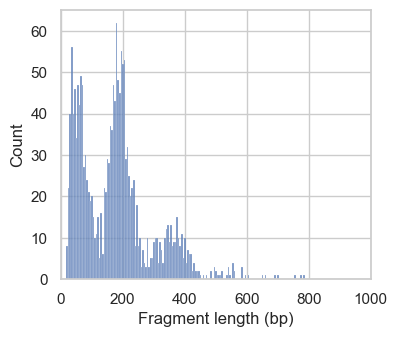
第一幅直方图显示逐渐减弱的周期性峰,分别对应短的无核小体片段,以及单、双和少量三核小体长度的片段。高质量数据通常富含短片段。这里 muon 的核小体信号以单核小体片段数为分子、无核小体片段数为分母;默认长度界限为 147 bp 和 294 bp,不能把图中约 100 bp 以下的短片段峰直接当作函数的阈值。第二组的比值偏高,因此本例将其排除。异常 Barcode 较少,提示该样本这一质量指标整体较好。
TSS 富集
信噪比还可通过峰内 Read 比例或 TSS 周围的信号富集来评估。本例使用后者。为兼顾计算时间与估计稳定性,随机抽取用于计算的 TSS 数量设为 n_tss=3000,高于这里所用实现的默认值 2,000。
tss = ac.tl.tss_enrichment(mdata, n_tss=3000, random_state=666)Fetching Regions...: 100%|██████████████████████████████████████████████████████████████████████████████████████████████████████████████████████████████████████████████| 3000/3000 [00:44<00:00, 67.37it/s]
该步骤创建 AnnData 对象 tss,以相对 TSS 的 −1,000 到 +1,000 bp 位置为 feature 汇总切割信号。同时将 tss_score 列写入 atac.obs 观测表。
分别展示全部 TSS 分数的分布,以及将显示范围限制到第 99.5 百分位数的分布;这一步只是调整绘图范围,尚未删除细胞。
fig, axs = plt.subplots(1, 2, figsize=(7, 3.5))

p1 = sns.histplot(atac.obs, x="tss_score", ax=axs[0])
p1.set_title("Full range")

p2 = sns.histplot(
    atac.obs,
    x="tss_score",
    binrange=(0, atac.obs["tss_score"].quantile(0.995)),
    ax=axs[1],
)
p2.set_title("Up to 99.5% percentile")

plt.suptitle("Distribution of the TSS score")

plt.tight_layout()
plt.show()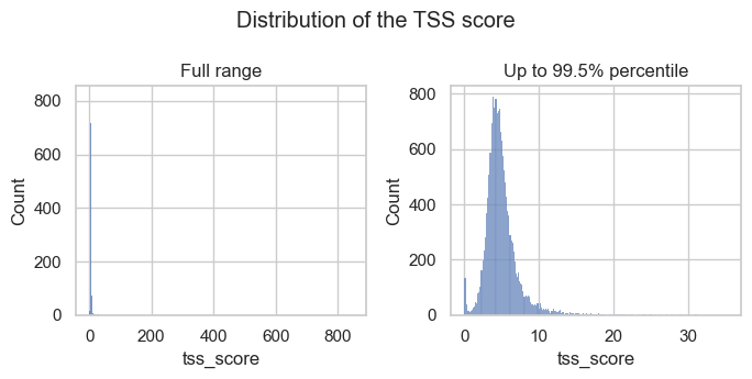
直方图中既有 TSS 分数极高的离群点,也有低分 Barcode 形成的小峰。本例后续将结合其他 QC 指标过滤这些观测。
为理解 TSS 分数,绘制 TSS 上下游的转座事件信号(片段末端)。调用 muon 的 ac.pl.tss_enrichment,传入刚生成的 tss 对象。随后按阈值区分前述低分小峰,在 tss.obs 中新建分组列,将细胞标为 "TSS_PASS" 或 "TSS_FAIL",比较两组的富集曲线。
tss_threshold = 1.5
tss.obs["tss_filter"] = [
    "TSS_FAIL" if score < tss_threshold else "TSS_PASS"
    for score in atac.obs["tss_score"]
]

# Print number cells not passing nucleosome signal threshold
tss.obs["tss_filter"].value_counts()
TSS_PASS 16483
TSS_FAIL 451
Name: tss_filter, dtype: int64# Temporarily set different color palette
sns.set_palette(palette="Set1")
ac.pl.tss_enrichment(tss, color="tss_filter")
# reset color palette
sns.set_palette(palette="tab10")/Users/christopher.lance/mambaforge/envs/scatac_pp/lib/python3.9/site-packages/muon/_atac/plot.py:282: FutureWarning: In a future version of pandas, a length 1 tuple will be returned when iterating over a groupby with a grouper equal to a list of length 1. Don't supply a list with a single grouper to avoid this warning.
for name, group in groups:
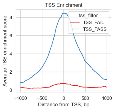
与高质量组相比,451 个低 TSS 分数细胞在 TSS 附近的富集明显减弱,提示信噪比较低。
查看当前对象,确认各项 QC 指标均已写入。
atacAnnData object with n_obs × n_vars = 16934 × 154027
obs: 'scDblFinder_score', 'AMULET_pVal', 'AMULET_qVal', 'AMULET_negLog10qVal', 'n_features_per_cell', 'total_fragment_counts', 'log_total_fragment_counts', 'nucleosome_signal', 'nuc_signal_filter', 'tss_score'
var: 'gene_ids', 'feature_types', 'genome', 'interval', 'n_cells_by_counts', 'mean_counts', 'pct_dropout_by_counts', 'total_counts'
uns: 'atac', 'files'过滤低质量细胞前,先保存包含 QC 指标的对象。
# save after calculation of QC metrics
atac.write_h5ad("output/atac_qc_metrics.h5ad")过滤细胞
不同样本的 QC 指标范围可能不同。应结合多种图形选择合理阈值,区分极端离群值与低质量细胞。
# Reload from file if needed
# atac = sc.read_h5ad("output/atac_qc_metrics.h5ad")
QC 指标的上限
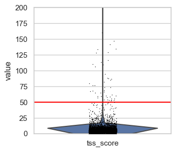
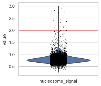
先查看 QC 指标的完整分布,寻找总 Count、TSS 分数或核小体信号异常偏高的 Barcode。下图的阈值线由本样本的初步诊断确定。
# Set thresholds for upper boundaries.
# These were identified by looking at the plots in this code cell before.
total_count_upper = 100000
tss_upper = 50
nucleosome_signal_upper = 2


# Plot total counts of fragments & features colored by TSS score
p1 = sc.pl.scatter(
    atac,
    x="total_fragment_counts",
    y="n_features_per_cell",
    size=40,
    color="tss_score",
    show=False,  # so that funstion output axis object where threshold line can be drawn.
)
p1.axvline(x=total_count_upper, c="red")  # Add vertical line

# tss.score
p2 = sc.pl.violin(atac, "tss_score", show=False)
p2.set_ylim(0, 200)  # zooming in a little to
p2.axhline(y=tss_upper, c="red")  # Add horizontal line

# nucleosome signal
p3 = sc.pl.violin(atac, "nucleosome_signal", show=False)
p3.axhline(y=nucleosome_signal_upper, c="red")

plt.show()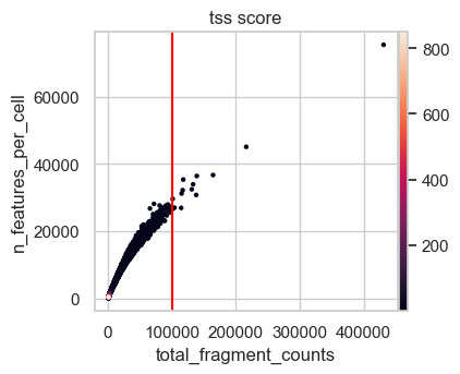
本例设置以下上限以排除极端离群值:
total_count_upper = 100000tss_upper = 50nucleosome_signal_upper = 2
feature 数与总 Count 高度相关,因此按总 Count 过滤通常也会去除 feature 数异常高的观测。TSS 富集较高通常是好现象,但极端值可能来自不稳定的背景估计或其他伪影。第一张散点图中,TSS 分数最高的 Barcode 反而具有很低的 Count 和 feature 数,说明需联合解读这些指标。
QC 指标的下限
为识别空液滴(empty droplet)和低质量细胞,绘制 scATAC-seq 中常用的散点图:横轴为总 Count 的对数,纵轴为 TSS 分数。
图中的阈值线根据本图及下方的补充诊断确定。
# upper TSS score boundary for plotting
plot_tss_max = 20

# Suggested thresholds (before log transform)
count_cutoff_lower = 1500
lcount_cutoff_upper = 100000
tss_cutoff_lower = 1.5
# Scatter plot & histograms
g = sns.jointplot(
data=atac[(atac.obs["tss_score"] < plot_tss_max)].obs,
x="log_total_fragment_counts",
y="tss_score",
color="black",
marker=".",
)
# Density plot including lines
g.plot_joint(sns.kdeplot, fill=True, cmap="Blues", zorder=1, alpha=0.75)
g.plot_joint(sns.kdeplot, color="black", zorder=2, alpha=0.75)
# Lines thresholds
plt.axvline(x=np.log10(count_cutoff_lower), c="red")
plt.axvline(x=np.log10(lcount_cutoff_upper), c="red")
plt.axhline(y=tss_cutoff_lower, c="red")
plt.show()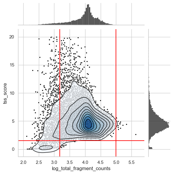
左下角有一群明显的低质量细胞,本例用 TSS 分数 1.5 作为下限将其排除。同时还需去除总 Count 分布左侧的低值尾部;具体阈值不总是清晰,宜结合其他图形判断。
与 scRNA-seq 类似,QC 阈值可能需要迭代调整。如果下游分析仍残留较多低质量细胞,或本应具有较低 Count、较少 feature 的细胞类型消失,应回到这里复核过滤条件。
下面绘制未经对数变换的总 Count 直方图,重点查看低值尾部。
fig, axs = plt.subplots(1, 2, figsize=(7, 3.5))

p1 = sns.histplot(
    atac.obs.loc[atac.obs["total_fragment_counts"] < 15000],
    x="total_fragment_counts",
    bins=40,
    ax=axs[0],
)
p1.set_title("< 15000")

p2 = sns.histplot(
    atac.obs.loc[atac.obs["total_fragment_counts"] < 3500],
    x="total_fragment_counts",
    bins=40,
    ax=axs[1],
)
p2.set_title("< 3500")
p2.axvline(x=1250, c="black", linestyle="--")
p2.axvline(x=1750, c="black", linestyle="--")

plt.suptitle("Total fragment count per cell")

plt.tight_layout()
plt.show()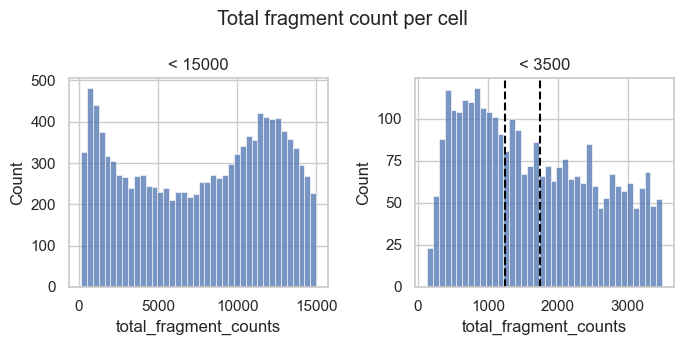
总 Count 较低的 Barcode 形成一个小峰,可能代表低质量观测。根据右图,可在约 1,250–1,750 之间选择下限以去除该峰。
再检查这一 Count 范围对应的 feature 数。图中以 1,500 作为参考,它位于上述建议范围的中间。
# Scatter plot total fragment count by number of features

n_feature_cutoff = 750  # added after looking at this plot

p2 = sc.pl.scatter(
    atac[atac.obs.total_fragment_counts < 3500],
    x="total_fragment_counts",
    y="n_features_per_cell",
    size=100,
    color="tss_score",
    show=False,
)
p2.axvline(x=count_cutoff_lower, c="red")
p2.axhline(y=n_feature_cutoff, c="red")

plt.show()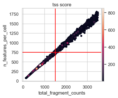
在图示低 Count 范围内,总 Count 与非零 feature 数接近线性关系。数据集共有超过 150,000 个 feature,本例认为至少检测到 750 个 feature 是较宽松的要求。综合这些诊断,将总 Count 下限设为 1,500;其他数据集仍需重新评估。
执行过滤
下方代码实际保留满足以下条件的细胞,边界值也包含在内:
每个细胞的总 Count:≥ 1,500 且 ≤ 100,000
每个细胞的 feature 数:≥ 750(本样本中约对应总 Count 1,500)
TSS 分数:≥ 1.5 且 ≤ 50
核小体信号:≤ 2
muon 可依据 .obs 中的任意一列过滤观测。
print(f"Total number of cells: {atac.n_obs}")
mu.pp.filter_obs(
    atac,
    "total_fragment_counts",
    lambda x: (x >= 1500) & (x <= 100000),
)
print(f"Number of cells after filtering on total_fragment_counts: {atac.n_obs}")
mu.pp.filter_obs(atac, "n_features_per_cell", lambda x: x >= 750)
print(f"Number of cells after filtering on n_features_per_cell: {atac.n_obs}")
Total number of cells: 16934
Number of cells after filtering on total_fragment_counts: 15386
Number of cells after filtering on n_features_per_cell: 15377
mu.pp.filter_obs(
    atac,
    "tss_score",
    lambda x: (x >= 1.5) & (x <= 50),
)
print(f"Number of cells after filtering on tss_score: {atac.n_obs}")
mu.pp.filter_obs(atac, "nucleosome_signal", lambda x: x <= 2)
print(f"Number of cells after filtering on nucleosome_signal: {atac.n_obs}")
Number of cells after filtering on tss_score: 15339
Number of cells after filtering on nucleosome_signal: 15286
过滤 feature
最后,去除仅在极少数细胞中检测到的 feature,以减少不稳定信号和下游计算开销。阈值需兼顾稀有细胞群体。
不同 scATAC-seq 工作流(workflow)可按检测到该 feature 的细胞数、细胞比例,或要保留的 feature 总数进行筛选;后者例如保留可及性最高的一部分 feature。
可用一个简单估算选择最小细胞数。假设目标稀有状态占全部细胞的 2%,其特异 feature 受随机漏检(dropout)影响,仅在该状态的 5% 细胞中被检测到。那么,这些 feature 平均只出现在全部细胞的 2% × 5% = 0.1% 中。对于约 15,000 个细胞的数据集,期望值仅为 15 个细胞。
本例据此采用 15 个细胞作为较宽松的最小检测数,以尽量保留稀有状态相关信号。这是结合研究目标的经验选择,并不保证所有保留的 feature 都具有可靠信号。
如果不研究稀有细胞类型或状态,可以提高阈值,例如仅保留至少在 1% 细胞中检测到的 feature,以进一步减少噪声与计算量。
muon 同样支持按变量列过滤 feature。注意,下方 n_cells_by_counts 是过滤细胞前计算的;若要求在保留的细胞中至少检测到 15 次,需先重新计算该列。
mu.pp.filter_var(atac, "n_cells_by_counts", lambda x: x >= 15)将过滤后的原始 Count 存入单独的层,供后续分析使用。下方赋值直接引用当前矩阵;若后续会就地修改同一矩阵,应显式复制以保留独立副本。
atac.layers["counts"] = atac.XatacAnnData object with n_obs × n_vars = 15286 × 154015
obs: 'scDblFinder_score', 'AMULET_pVal', 'AMULET_qVal', 'AMULET_negLog10qVal', 'n_features_per_cell', 'total_fragment_counts', 'log_total_fragment_counts', 'nucleosome_signal', 'nuc_signal_filter', 'tss_score'
var: 'gene_ids', 'feature_types', 'genome', 'interval', 'n_cells_by_counts', 'mean_counts', 'pct_dropout_by_counts', 'total_counts'
uns: 'atac', 'files'
layers: 'counts'最后保存过滤后的 ATAC 对象,用于后续降维(dimensionality reduction)。
atac.write_h5ad("output/atac_qc_filtered.h5ad")- Chen, H., Lareau, C., Andreani, T., Vinyard, M. E., Garcia, S. P., Clement, K., Andrade-Navarro, M. A., Buenrostro, J. D., & Pinello, L. (2019). Assessment of computational methods for the analysis of single-cell ATAC-seq data. Genome Biology, 20(1), 241. 10.1186/s13059-019-1854-5
- Luecken, M. D., Burkhardt, D. B., Cannoodt, R., Lance, C., Agrawal, A., Aliee, H., Chen, A. T., Deconinck, L., Detweiler, A. M., Granados, A. A., Huynh, S., Isacco, L., Kim, Y. J., Klein, D., KUMAR, B. D., Kuppasani, S., Lickert, H., McGeever, A., Mekonen, H., … Bloom, J. M. (2021). A sandbox for prediction and integration of DNA, RNA, and proteins in single cells. Thirty-Fifth Conference on Neural Information Processing Systems Datasets and Benchmarks Track (Round 2). https://openreview.net/forum?id=gN35BGa1Rt
- Germain, P.-L., Lun, A., Meixide, C. G., Macnair, W., & Robinson, M. D. (2021). Doublet identification in single-cell sequencing data using scDblFinder. F1000Research, 10.
- Thibodeau, A., Eroglu, A., McGinnis, C. S., Lawlor, N., Nehar-Belaid, D., Kursawe, R., Marches, R., Conrad, D. N., Kuchel, G. A., Gartner, Z. J., Banchereau, J., Stitzel, M. L., Cicek, A. E., & Ucar, D. (2021). AMULET: a novel read count-based method for effective multiplet detection from single nucleus ATAC-seq data. Genome Biology, 22(1), 252. 10.1186/s13059-021-02469-x
- Thibodeau, A., Eroglu, A., & Ucar, D. (2021). AMULET: a novel read count-based method for effective multiplet detection from single nucleus ATAC-seq data. Zenodo. 10.5281/ZENODO.5189588