克隆型分析 - 单细胞最佳实践

步骤

yml

安装 conda：
- 在创建环境之前，请确保 conda 已安装在你的系统中。
保存 yml 内容：
- 将 yml 选项卡中的内容保存为文件 environment.yml。
创建环境：
- 打开终端或命令提示符。
- 运行以下命令：
```
conda env create -f environment.yml
```
激活环境：
- 创建好环境后，使用以下命令激活它：
```
conda activate <environment_name>
```
- 请将 <environment_name> 替换为 environment.yml 文件中指定的环境名称。该名称在 yml 文件中如下所示：
```
name: <environment_name>
```
验证安装：
- 通过运行以下命令，检查环境是否创建成功：
```
conda env list
```

克隆扩增：多样性与丰度¶

静息淋巴细胞在抗原识别及相关信号刺激下可活化并大量增殖，这一过程称为克隆扩增（clonal expansion）。细胞因子等刺激既可来自细胞自身，也可来自其他细胞；“来自同一机体”并不等同于自分泌 Polonsky et al., 2016。在单细胞数据中，多个细胞携带相同的免疫受体（Immune Receptor, IR），可作为识别扩增克隆的依据。这些信息有助于研究初始淋巴细胞向效应或记忆状态的转变，并与细胞注释结合解释 Polonsky et al., 2016。分析时还应考虑克隆竞争（clonal competition）（不同克隆争夺有限资源）、克隆优势（clonal dominance）（少数克隆占据较高比例）及旁观者激活（bystander activation）（细胞因子驱动 T 细胞活化，而非由其受体直接识别相应抗原）等过程 Naxerova, 2020Ashcroft et al., 2017Kim & Shin, 2019。

克隆型（clonotype）及其细胞数可以借用群落生态学中的多样性（diversity）与丰度（abundance）概念描述。多样性综合反映类别数及其分布均匀程度；丰度则描述某一类别的个体数或相对频率 Travlos et al., 2018。在 IR 分析中，将“物种”替换为“克隆型”、“个体”替换为“细胞”即可。少数克隆大量扩增时，其丰度和群体占比增加，受体库的均匀度常会下降。例如，效应 CD8+ T 细胞中可能出现优势克隆。但这不意味着不同克隆的实际种类必然减少；观测多样性还受到采样深度和所用指标的影响。

基因片段使用与谱型¶

T 细胞受体（T-Cell Receptor, TCR）和 B 细胞受体（B-Cell Receptor, BCR）的可变区由可变（variable, V）、多样性（diversity, D）及连接（joining, J）基因片段重组而成。重组具有随机性，但并不意味着所有序列或片段组合等概率。不同个体间可观察到一些相近的 V(D)J 基因片段使用（gene segment usage）模式，提示生成机制与后续选择存在偏好 Elhanati et al., 2014。可以分别比较不同细胞类型、不同个体中各片段的使用频率 Chernyshev et al., 2021，并结合受体序列及基因注释考察 V(D)J 组合。单凭氨基酸组成通常不能唯一确定所有基因片段来源。

V(D)J 重组中的片段连接及核苷酸插入、切除，使互补决定区 3（Complementarity-Determining Region 3, CDR3）的长度发生变化。谱型分析（spectratype analysis）通过 CDR3 或所记录连接区的长度分布描述受体库的异质性 Ciupe et al., 2013。结合克隆扩增和基因使用分析，可以进一步刻画优势克隆；长度相同本身并不能证明属于同一克隆或具有同一抗原特异性。

TCR 数据准备¶

与预处理阶段一样，这里使用 Scirpy 完成分析，并将结果保存在 AnnData 对象中。

import warnings

warnings.filterwarnings(
    "ignore",
    ".*IProgress not found*",
)
warnings.simplefilter(action="ignore", category=FutureWarning)

import numpy as np
import pandas as pd
import scanpy as sc
import scirpy as ir
from palmotif import compute_motif, svg_logo

warnings.simplefilter(action="ignore", category=pd.errors.DtypeWarning)

sc.logging.print_versions()

WARNING: If you miss a compact list, please try `print_header`!
-----
anndata     0.8.0
scanpy      1.6.1
sinfo       0.3.1
-----
Levenshtein                 NA
PIL                         8.1.0
adjustText                  NA
airr                        1.3.1
anndata                     0.8.0
anyio                       NA
attr                        20.3.0
babel                       2.9.0
backcall                    0.2.0
brotli                      1.0.9
certifi                     2020.12.05
cffi                        1.14.4
chardet                     4.0.0
cloudpickle                 1.6.0
constants                   NA
cycler                      0.10.0
cython_runtime              NA
dask                        2020.12.0
dateutil                    2.8.1
decorator                   4.4.2
future_fstrings             NA
get_version                 2.1
google                      NA
h5py                        3.7.0
highs_wrapper               NA
idna                        2.10
igraph                      0.8.3
ipykernel                   5.4.3
ipython_genutils            0.2.0
ipywidgets                  7.6.3
jedi                        0.18.0
jinja2                      2.11.2
joblib                      1.0.0
json5                       NA
jsonschema                  3.2.0
jupyter_server              1.2.1
jupyterlab_server           2.1.2
kiwisolver                  1.3.1
legacy_api_wrap             1.2
leidenalg                   0.8.3
llvmlite                    0.35.0
louvain                     0.7.0
lxml                        4.6.2
markupsafe                  1.1.1
matplotlib                  3.3.3
mpl_toolkits                NA
natsort                     7.1.0
nbclassic                   NA
nbformat                    5.1.1
networkx                    2.5
numba                       0.52.0
numexpr                     2.7.2
numpy                       1.19.5
packaging                   20.8
pandas                      1.2.0
parasail                    1.2.4
parso                       0.8.1
pexpect                     4.8.0
pickleshare                 0.7.5
pkg_resources               NA
prometheus_client           NA
prompt_toolkit              3.0.10
ptyprocess                  0.7.0
pvectorc                    NA
pygments                    2.7.4
pyparsing                   2.4.7
pyrsistent                  NA
pytz                        2020.5
requests                    2.25.1
scanpy                      1.6.1
scipy                       1.6.0
scirpy                      0.11.0
seaborn                     0.11.1
send2trash                  NA
setuptools_scm              NA
sinfo                       0.3.1
six                         1.15.0
sklearn                     0.24.0
sniffio                     1.2.0
sparse                      0.11.2
statsmodels                 0.12.1
storemagic                  NA
tables                      3.6.1
texttable                   1.6.3
tlz                         0.11.1
toolz                       0.11.1
tornado                     6.1
tqdm                        4.56.0
tracerlib                   NA
traitlets                   5.0.5
typing_extensions           NA
urllib3                     1.26.2
wcwidth                     0.2.5
yaml                        5.3.1
yamlordereddictloader       NA
zmq                         21.0.0
-----
IPython             7.19.0
jupyter_client      6.1.11
jupyter_core        4.7.0
jupyterlab          3.0.4
notebook            6.2.0
-----
Python 3.8.6 (default, Jan 14 2021, 17:39:54) [GCC 8.3.0]
Linux-3.10.0-1160.25.1.el7.x86_64-x86_64-with-glibc2.28
48 logical CPU cores
-----
Session information updated at 2022-08-12 11:05

path_data = "/home/icb/juan.henao/BestPracticeStart/data"

path_gex = f"{path_data}/TCR_filtered.h5ad"
adata = sc.read(path_gex)

说明

为控制演示所需的计算量和运行时间，下面使用原始数据的一个子集。

我们选取六名参与者的样本，覆盖不同采集中心和临床状态。

adata = adata[
    adata.obs["patient_id"].isin(
        ["COVID-014", "CV0902", "AP6", "COVID-045", "COVID-066", "COVID-067"]
    )
]
# adata[adata.obs['Status'] == 'Healthy'].obs['patient_id']
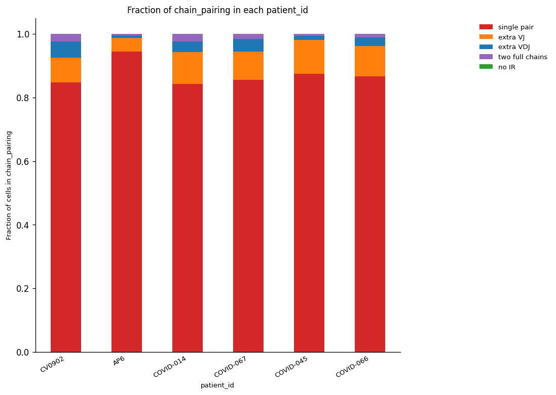
_ = ir.pl.group_abundance(
    adata,
    groupby="patient_id",
    target_col="chain_pairing",
    normalize=True,
    figsize=[10, 10],
)

/home/juan.henao/.local/lib/python3.8/site-packages/anndata/compat/_overloaded_dict.py:106: ImplicitModificationWarning: Trying to modify attribute `._uns` of view, initializing view as actual.
  self.data[key] = value

克隆型定义¶

常见的克隆型定义，是将 VJ 链和 VDJ 链的 CDR3 序列均相同的细胞归为一组。需要明确比较的是核苷酸还是氨基酸：本例使用氨基酸相同，趋同重组产生的不同核苷酸序列仍可能归入一组，因此不能将结果直接等同于已确证的细胞谱系。也可以根据序列距离和阈值，将相近受体归为克隆型簇；其含义取决于所选距离及匹配规则。

ir.pp.ir_dist(adata, sequence="aa")

计算 CDR3 的序列匹配关系后，可以据此对细胞分组。定义时可以要求 VJ 和 VDJ 两类链都匹配，也可以只比较其中一类；对具有额外链的细胞，还可以选择仅使用主链，或纳入次要链。不同设置对应不同的克隆型定义，应根据研究目的明确记录。

克隆型分组的序列类型和距离度量必须与前一步一致。本例使用氨基酸序列及默认的 identity 度量；receptor_arms="all" 要求所比较的 VJ/VDJ 链均匹配，dual_ir="primary_only" 仅使用按链丰度等规则选出的主链。

ir.tl.define_clonotype_clusters(
    adata, sequence="aa", receptor_arms="all", dual_ir="primary_only"
)

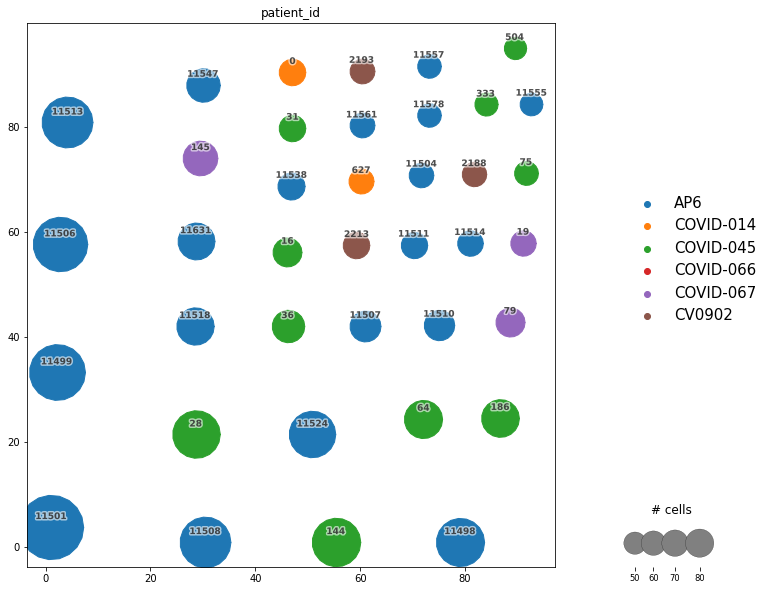
可用网络展示分组结果，节点表示共享受体配置的细胞，节点大小反映相应细胞数。在本例的严格 identity 定义下，图中分组对应克隆型。数字 ID 只是标签，不表示克隆大小、出现时间或其他生物学顺序。

绘图前先计算网络布局，Scirpy 提供相应的布局选项。为了避免只有一个细胞的克隆型（singleton）占满画面，通常可将 min_cells 设为至少 2。本例设为 50，仅展示至少包含 50 个细胞的分组，便于观察较大的克隆型；这一设置用于绘图筛选。

ir.tl.clonotype_network(adata, min_cells=50, sequence="aa")

计算布局后即可绘图。本例中，圆形节点及其编号用于定位克隆型，节点大小对应所包含的细胞数。

按参与者着色可查看克隆型是否跨样本出现。通常将不同个体间共享的克隆型称为 公共克隆型（public clonotypes），它们可能反映共有的免疫识别，也可能受到受体生成概率等因素影响，不能仅凭共享就归因于同一疾病。仅在某一个体中检出的则称为 私有克隆型（private clonotypes），可用于研究个体特异的受体库特征。本例图中的最大克隆型分别由单一参与者的细胞组成；未在其他样本检出也受到采样深度限制。

_ = ir.pl.clonotype_network(
    adata,
    color="patient_id",
    base_size=10,
    label_fontsize=9,
    panel_size=(10, 10),
    legend_fontsize=15,
)

... storing 'cc_aa_identity' as categorical

adata.obs["cc_aa_identity"] = adata.obs["cc_aa_identity"].astype("str")

克隆型 ID 可用于提取具体记录。下面查看 0 号克隆型的受体序列、受体亚型和对应细胞数。

adata.obs.loc[adata.obs["cc_aa_identity"] == "0", :].groupby(
    [
        "IR_VJ_1_junction_aa",
        "IR_VDJ_1_junction_aa",
        "receptor_subtype",
    ],
    observed=True,
).size().reset_index(name="n_cells")

克隆扩增¶

免疫刺激可促使特定淋巴细胞增殖，使某些克隆型在样本中出现多次。下面按克隆型细胞数标记扩增程度，并把结果加入 .obs。这是对当前样本的描述，不是直接测量细胞分裂，也不应与胸腺发育中的“正选择”混为一谈。

随后按细胞类型绘制堆叠柱状图，显示各扩增类别中的细胞数。图中的统计单位是细胞，不是不同克隆型的个数。

ir.tl.clonal_expansion(adata, target_col="cc_aa_identity")

_ = ir.pl.clonal_expansion(
    adata,
    groupby="initial_clustering",
    target_col="cc_aa_identity",
    clip_at=4,
    normalize=False,
    figsize=[10, 10],
)

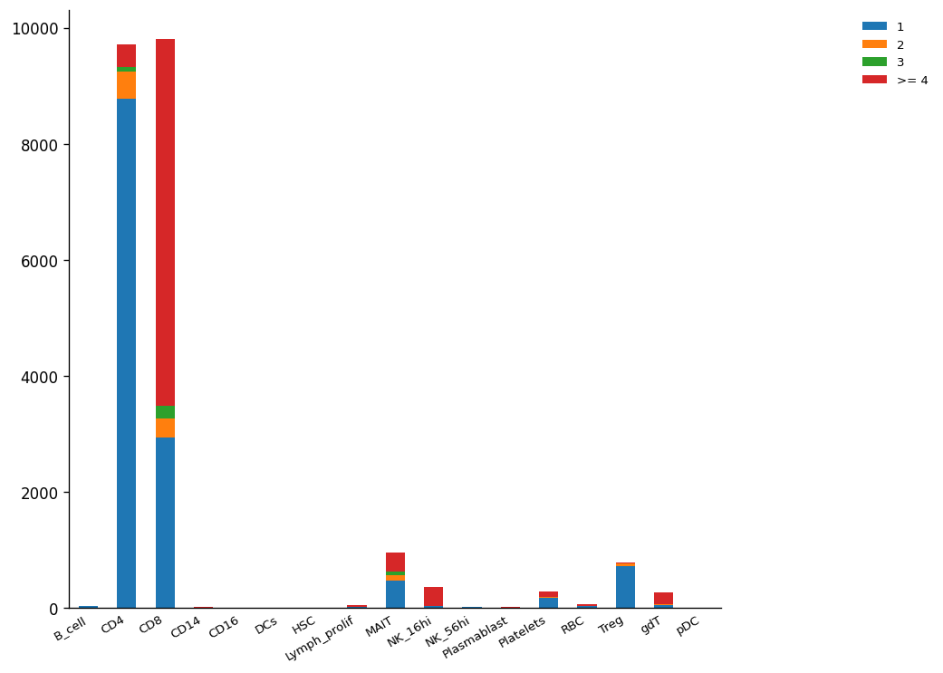
本例图中 CD4+ T 细胞总数最多，而 CD8+ 群体中属于扩增克隆的细胞较多，与效应 T 细胞扩增的解释相符。不能仅由这张图确定扩增的刺激来源。

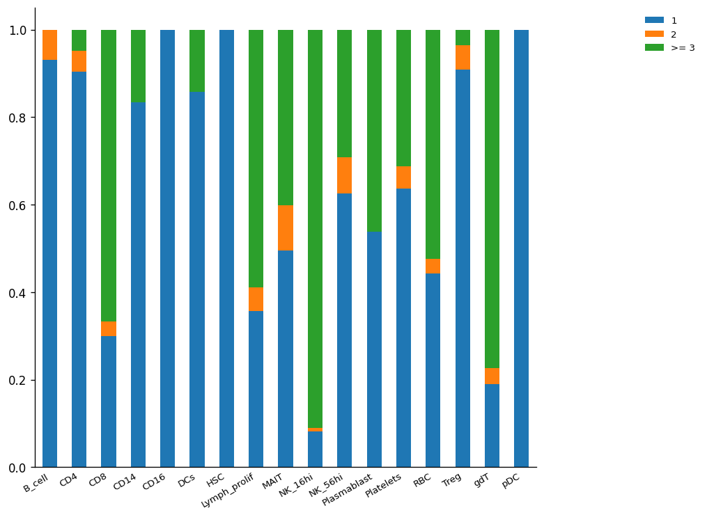
将各细胞类型的总量归一化为比例后，可以更清楚地比较 CD4+ 与 CD8+ 群体的扩增组成。

_ = ir.pl.clonal_expansion(
    adata, "initial_clustering", target_col="cc_aa_identity", figsize=[10, 10]
)

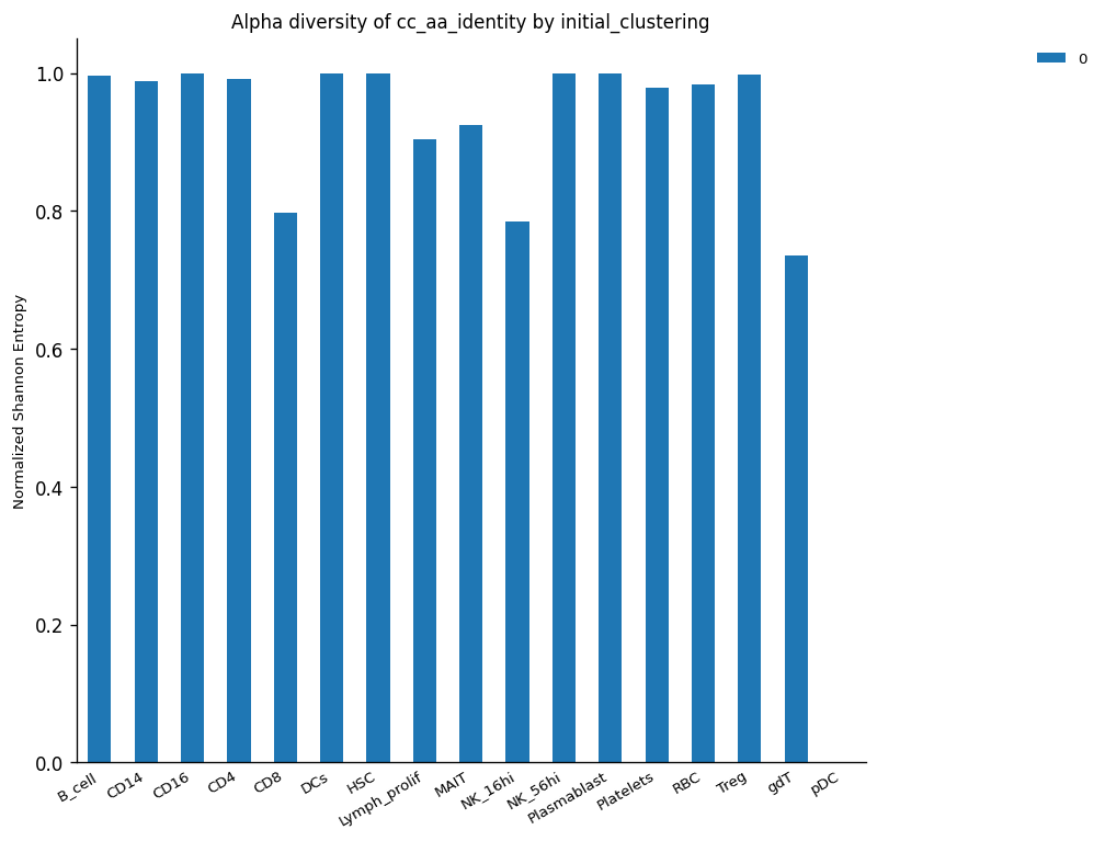
还可通过 α 多样性（alpha diversity）描述一个样本或细胞群内部的克隆型多样性。当少数克隆占据较大比例时，反映均匀度的指标通常下降。不同多样性指标对稀有克隆和优势克隆的权重不同，因此应明确所用指标，并考虑细胞采样量差异。

本例中 CD8+ 群体的 α 多样性低于 CD4+，与前面的扩增模式相符。原注释中的 NK_16hi 和 gdT-cell 群体也显示较低多样性，但这些是继承的转录组标签：尤其是 NK 标签下出现 TCR 时，应核对细胞注释、受体类型及潜在双细胞（Doublet），不能据此声称常规 NK 细胞具有重排的 TCR 克隆。

_ = ir.pl.alpha_diversity(
    adata, groupby="initial_clustering", target_col="cc_aa_identity", figsize=[10, 10]
)

克隆型丰度¶

克隆扩增会增加该克隆的细胞数，常伴随其相对丰度升高；群体多样性的变化则取决于整体克隆组成，二者并非简单互为反义。

下面显示细胞数最多的十个克隆型，列出其 ID，并按细胞类型分解各克隆的细胞组成。

_ = ir.pl.group_abundance(
    adata,
    groupby="cc_aa_identity",
    target_col="initial_clustering",
    max_cols=10,
    figsize=[10, 10],
)

... storing 'cc_aa_identity' as categorical
... storing 'clonal_expansion' as categorical
Using categorical units to plot a list of strings that are all parsable as floats or dates. If these strings should be plotted as numbers, cast to the appropriate data type before plotting.
Using categorical units to plot a list of strings that are all parsable as floats or dates. If these strings should be plotted as numbers, cast to the appropriate data type before plotting.
Using categorical units to plot a list of strings that are all parsable as floats or dates. If these strings should be plotted as numbers, cast to the appropriate data type before plotting.
Using categorical units to plot a list of strings that are all parsable as floats or dates. If these strings should be plotted as numbers, cast to the appropriate data type before plotting.
Using categorical units to plot a list of strings that are all parsable as floats or dates. If these strings should be plotted as numbers, cast to the appropriate data type before plotting.
Using categorical units to plot a list of strings that are all parsable as floats or dates. If these strings should be plotted as numbers, cast to the appropriate data type before plotting.
Using categorical units to plot a list of strings that are all parsable as floats or dates. If these strings should be plotted as numbers, cast to the appropriate data type before plotting.
Using categorical units to plot a list of strings that are all parsable as floats or dates. If these strings should be plotted as numbers, cast to the appropriate data type before plotting.
Using categorical units to plot a list of strings that are all parsable as floats or dates. If these strings should be plotted as numbers, cast to the appropriate data type before plotting.
Using categorical units to plot a list of strings that are all parsable as floats or dates. If these strings should be plotted as numbers, cast to the appropriate data type before plotting.
Using categorical units to plot a list of strings that are all parsable as floats or dates. If these strings should be plotted as numbers, cast to the appropriate data type before plotting.
Using categorical units to plot a list of strings that are all parsable as floats or dates. If these strings should be plotted as numbers, cast to the appropriate data type before plotting.
Using categorical units to plot a list of strings that are all parsable as floats or dates. If these strings should be plotted as numbers, cast to the appropriate data type before plotting.
Using categorical units to plot a list of strings that are all parsable as floats or dates. If these strings should be plotted as numbers, cast to the appropriate data type before plotting.
Using categorical units to plot a list of strings that are all parsable as floats or dates. If these strings should be plotted as numbers, cast to the appropriate data type before plotting.
Using categorical units to plot a list of strings that are all parsable as floats or dates. If these strings should be plotted as numbers, cast to the appropriate data type before plotting.
Using categorical units to plot a list of strings that are all parsable as floats or dates. If these strings should be plotted as numbers, cast to the appropriate data type before plotting.
Using categorical units to plot a list of strings that are all parsable as floats or dates. If these strings should be plotted as numbers, cast to the appropriate data type before plotting.
Using categorical units to plot a list of strings that are all parsable as floats or dates. If these strings should be plotted as numbers, cast to the appropriate data type before plotting.
Using categorical units to plot a list of strings that are all parsable as floats or dates. If these strings should be plotted as numbers, cast to the appropriate data type before plotting.
Using categorical units to plot a list of strings that are all parsable as floats or dates. If these strings should be plotted as numbers, cast to the appropriate data type before plotting.
Using categorical units to plot a list of strings that are all parsable as floats or dates. If these strings should be plotted as numbers, cast to the appropriate data type before plotting.
Using categorical units to plot a list of strings that are all parsable as floats or dates. If these strings should be plotted as numbers, cast to the appropriate data type before plotting.
Using categorical units to plot a list of strings that are all parsable as floats or dates. If these strings should be plotted as numbers, cast to the appropriate data type before plotting.
Using categorical units to plot a list of strings that are all parsable as floats or dates. If these strings should be plotted as numbers, cast to the appropriate data type before plotting.
Using categorical units to plot a list of strings that are all parsable as floats or dates. If these strings should be plotted as numbers, cast to the appropriate data type before plotting.
Using categorical units to plot a list of strings that are all parsable as floats or dates. If these strings should be plotted as numbers, cast to the appropriate data type before plotting.
Using categorical units to plot a list of strings that are all parsable as floats or dates. If these strings should be plotted as numbers, cast to the appropriate data type before plotting.
Using categorical units to plot a list of strings that are all parsable as floats or dates. If these strings should be plotted as numbers, cast to the appropriate data type before plotting.
Using categorical units to plot a list of strings that are all parsable as floats or dates. If these strings should be plotted as numbers, cast to the appropriate data type before plotting.
Using categorical units to plot a list of strings that are all parsable as floats or dates. If these strings should be plotted as numbers, cast to the appropriate data type before plotting.
Using categorical units to plot a list of strings that are all parsable as floats or dates. If these strings should be plotted as numbers, cast to the appropriate data type before plotting.
Using categorical units to plot a list of strings that are all parsable as floats or dates. If these strings should be plotted as numbers, cast to the appropriate data type before plotting.
Using categorical units to plot a list of strings that are all parsable as floats or dates. If these strings should be plotted as numbers, cast to the appropriate data type before plotting.

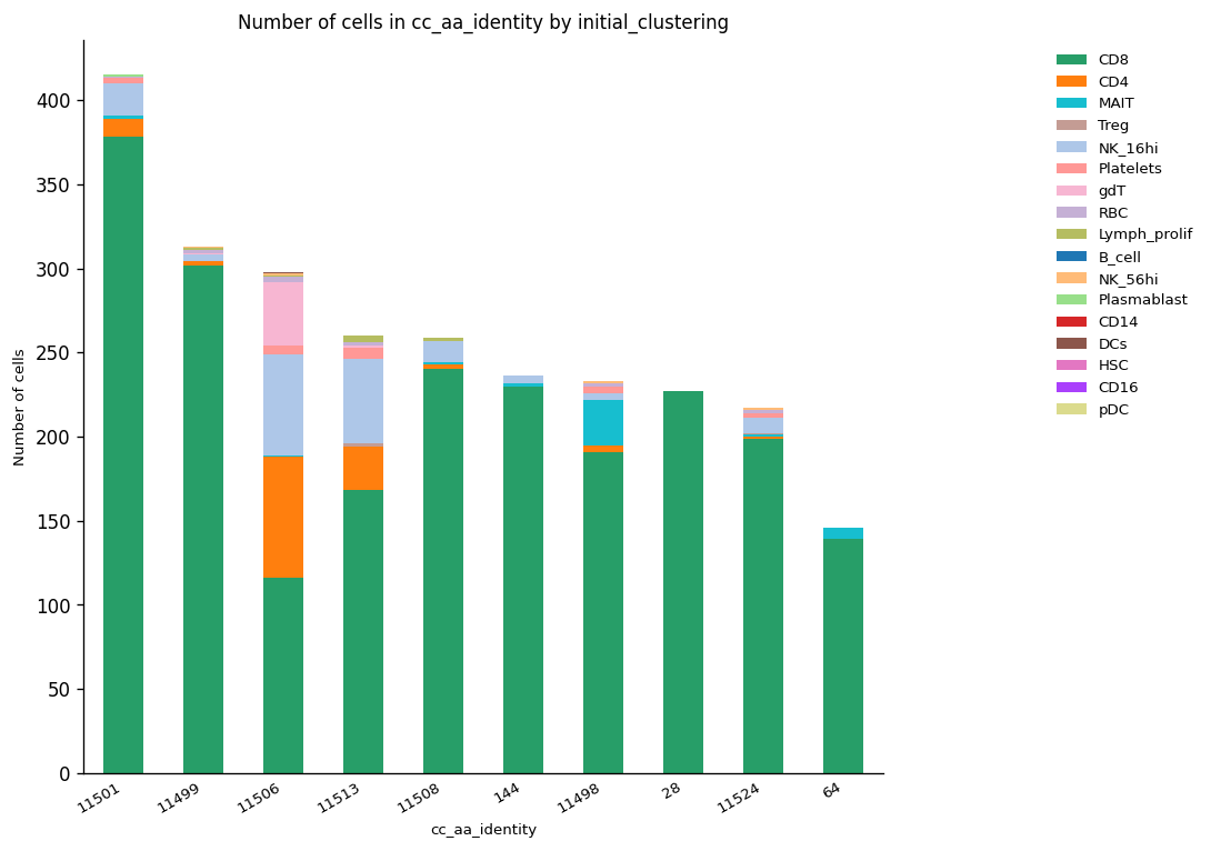
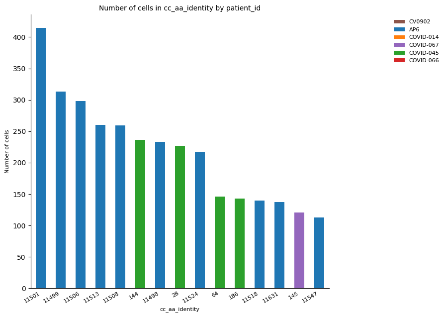
原教程图中，11501 号克隆型细胞数最多，并分布于多个转录组细胞簇。可以进一步按参与者和临床状态着色，核对这些细胞是否来自同一样本及同一条件；克隆型 ID 本身不包含这类信息。

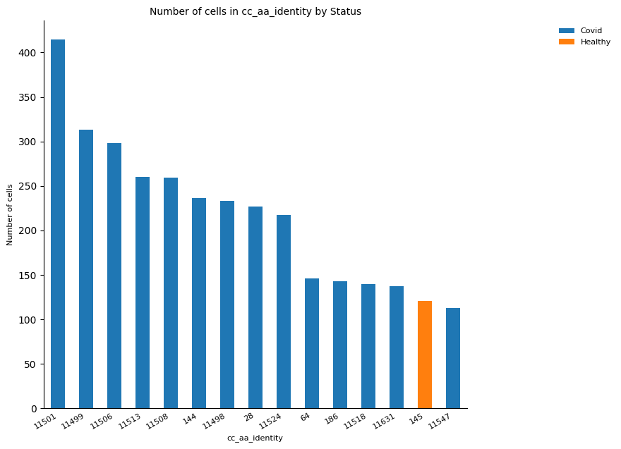
感染相关免疫应答可能伴随克隆扩增，因此可以检查较大克隆是否富集于 COVID 样本。但健康个体也可能携带已扩增的记忆克隆，不能预先认定全部或多数最大克隆必然来自 COVID 患者。

# By condition

_ = ir.pl.group_abundance(
    adata,
    groupby="cc_aa_identity",
    target_col="Status",
    max_cols=15,
    fig_kws={"dpi": 100},
    figsize=[10, 10],
)

# By sample

_ = ir.pl.group_abundance(
    adata,
    groupby="cc_aa_identity",
    target_col="patient_id",
    max_cols=15,
    fig_kws={"dpi": 100},
    figsize=[10, 10],
)

Using categorical units to plot a list of strings that are all parsable as floats or dates. If these strings should be plotted as numbers, cast to the appropriate data type before plotting.
Using categorical units to plot a list of strings that are all parsable as floats or dates. If these strings should be plotted as numbers, cast to the appropriate data type before plotting.
Using categorical units to plot a list of strings that are all parsable as floats or dates. If these strings should be plotted as numbers, cast to the appropriate data type before plotting.
Using categorical units to plot a list of strings that are all parsable as floats or dates. If these strings should be plotted as numbers, cast to the appropriate data type before plotting.
Using categorical units to plot a list of strings that are all parsable as floats or dates. If these strings should be plotted as numbers, cast to the appropriate data type before plotting.
Using categorical units to plot a list of strings that are all parsable as floats or dates. If these strings should be plotted as numbers, cast to the appropriate data type before plotting.
Using categorical units to plot a list of strings that are all parsable as floats or dates. If these strings should be plotted as numbers, cast to the appropriate data type before plotting.
Using categorical units to plot a list of strings that are all parsable as floats or dates. If these strings should be plotted as numbers, cast to the appropriate data type before plotting.
Using categorical units to plot a list of strings that are all parsable as floats or dates. If these strings should be plotted as numbers, cast to the appropriate data type before plotting.
Using categorical units to plot a list of strings that are all parsable as floats or dates. If these strings should be plotted as numbers, cast to the appropriate data type before plotting.
Using categorical units to plot a list of strings that are all parsable as floats or dates. If these strings should be plotted as numbers, cast to the appropriate data type before plotting.
Using categorical units to plot a list of strings that are all parsable as floats or dates. If these strings should be plotted as numbers, cast to the appropriate data type before plotting.
Using categorical units to plot a list of strings that are all parsable as floats or dates. If these strings should be plotted as numbers, cast to the appropriate data type before plotting.
Using categorical units to plot a list of strings that are all parsable as floats or dates. If these strings should be plotted as numbers, cast to the appropriate data type before plotting.
Using categorical units to plot a list of strings that are all parsable as floats or dates. If these strings should be plotted as numbers, cast to the appropriate data type before plotting.
Using categorical units to plot a list of strings that are all parsable as floats or dates. If these strings should be plotted as numbers, cast to the appropriate data type before plotting.

基因使用¶

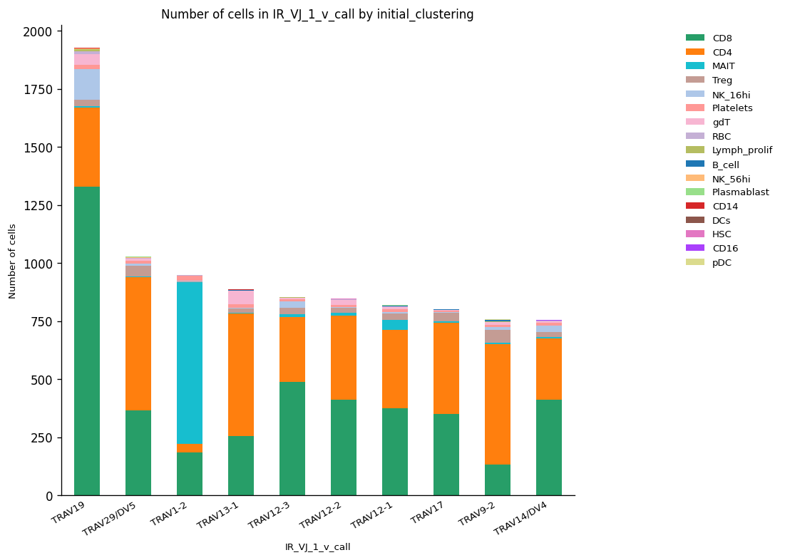
除克隆型、多样性和丰度外，还可分析具体 V(D)J 基因片段在各细胞簇中的使用情况，以及这些片段如何组合形成受体。

先统计各基因片段对应的细胞数，找出在样本中使用较多的片段。这是观测使用频率，既受重组和选择影响，也受克隆扩增、细胞组成及采样影响；高丰度不能单独证明该片段在重组时被优先选择。

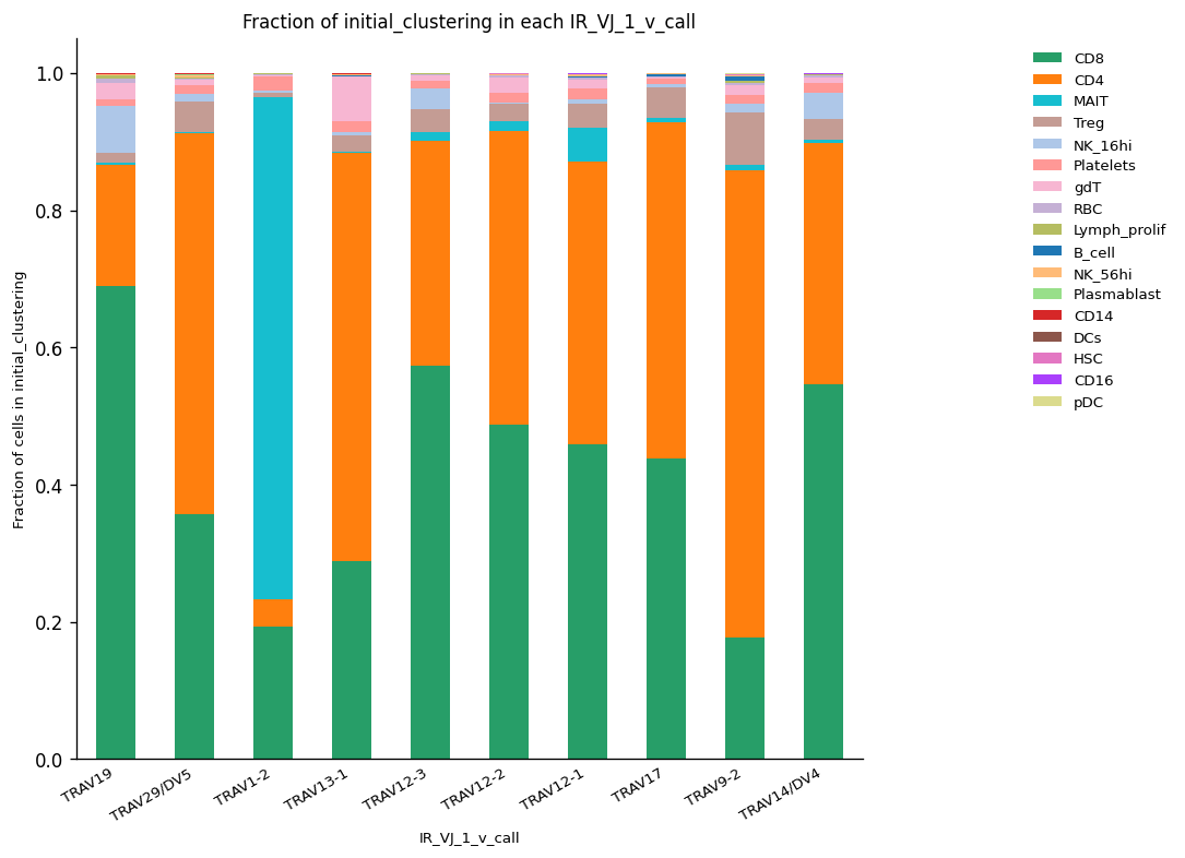
这里沿用丰度绘图函数，统计 VJ 主链的 V 基因使用。原教程中 TRAV19 对应的细胞最多，主要属于 CD8+；其次为 TRAV29/DV5，主要属于 CD4+。归一化图展示各基因对应细胞的类型组成。

_ = ir.pl.group_abundance(
    adata,
    groupby="IR_VJ_1_v_call",
    target_col="initial_clustering",
    normalize=False,
    max_cols=10,
    figsize=[10, 10],
)

# Normalized abundances

_ = ir.pl.group_abundance(
    adata,
    groupby="IR_VJ_1_v_call",
    target_col="initial_clustering",
    normalize=True,
    max_cols=10,
    figsize=[10, 10],
)

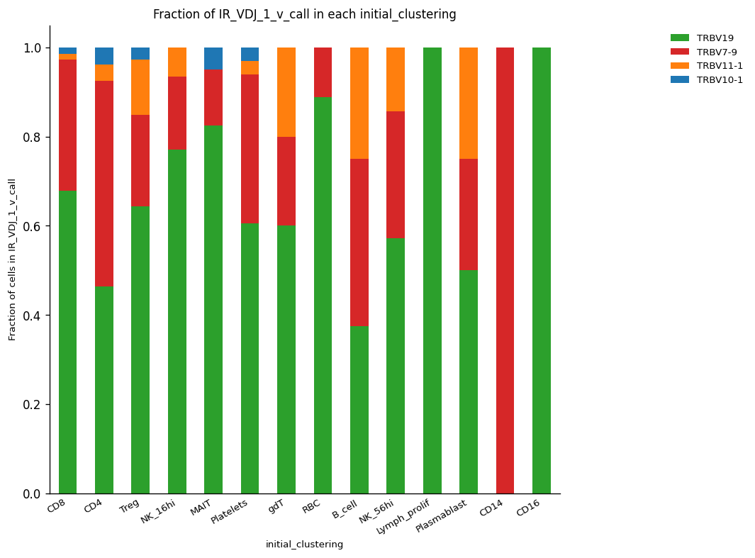
也可以先选择感兴趣的基因，再按细胞类型查看这些基因在所选子集中的相对比例。

下面实际选择的四个 VDJ 链 V 基因为 TRBV19、TRBV10-1、TRBV11-1 和 TRBV7-9。原文在此提到 TRBV18，但它不在代码的筛选列表中，不能据此描述本图的优势基因。

_ = ir.pl.group_abundance(
    adata[
        adata.obs["IR_VDJ_1_v_call"].isin(
            ["TRBV19", "TRBV10-1", "TRBV11-1", "TRBV7-9"]
        ),
        :,
    ],
    groupby="initial_clustering",
    target_col="IR_VDJ_1_v_call",
    normalize=True,
    figsize=[10, 10],
)

/home/juan.henao/.local/lib/python3.8/site-packages/anndata/compat/_overloaded_dict.py:106: ImplicitModificationWarning: Trying to modify attribute `._uns` of view, initializing view as actual.
  self.data[key] = value

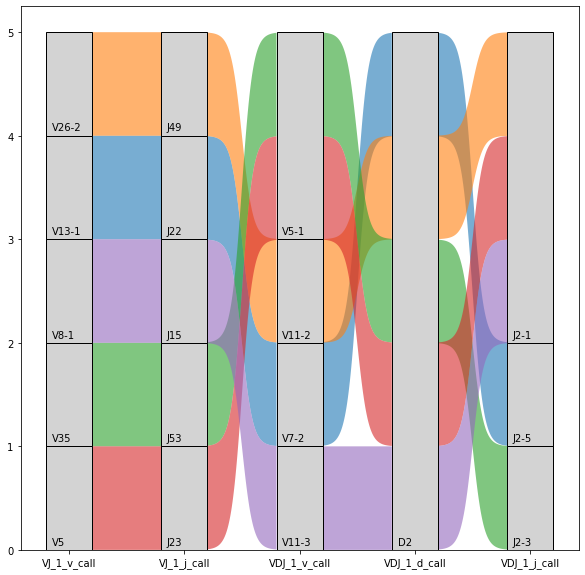
除了单个基因片段的丰度，还可以用连接图展示 V、D、J 片段的组合。这有助于观察 α、β 链中常见片段与其他片段的搭配，以及不同组合的相对规模。

某个片段单独出现频繁，并不意味着它一定与另一个高频片段组合。片段的联合使用需要从实际组合中统计；随机重组也不自动意味着所有片段彼此独立或等概率。

_ = ir.pl.vdj_usage(
    adata,
    full_combination=False,
    max_segments=None,
    max_ribbons=30,
    fig_kws={"figsize": [10, 10]},
)

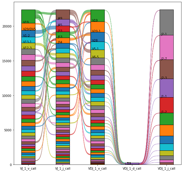
原教程的这张图只显示了 TRBD2 这一 D 基因注释。该现象仅描述所选数据和可用注释，不能推断人类 TCR β 链只使用一个 D 基因。

也可以先选择特定细胞或克隆型，再绘制片段组合。下面统计带 TRBD2 注释的克隆型，并选取列出的五个克隆型 ID 进行展示；这些 ID 是当前分组结果中的标签。

adata.obs[adata.obs["IR_VDJ_1_d_call"] == "TRBD2"].cc_aa_identity.value_counts()

5150     1
1815     1
4427     1
3500     1
4078     1
        ..
4734     0
4735     0
4736     0
4737     0
14180    0
Name: cc_aa_identity, Length: 14181, dtype: int64

_ = ir.pl.vdj_usage(
    adata[
        adata.obs["cc_aa_identity"].isin(["5150", "1815", "4427", "3500", "4078"]), :
    ],
    max_ribbons=None,
    max_segments=100,
    fig_kws={"figsize": [10, 10]},
)

谱型分析¶

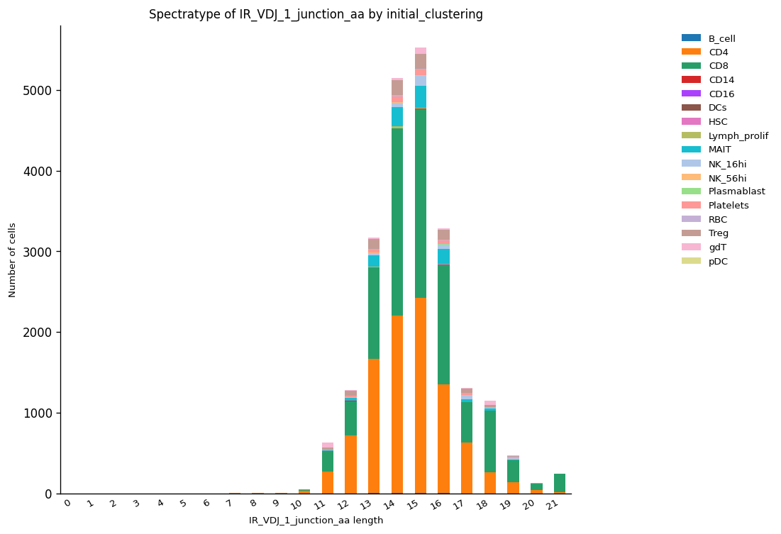
谱型分析考察连接区长度分布，补充受体序列异质性的信息。重组连接处的插入和切除会产生不同长度；本例使用 junction_aa 字段，测量的是 CDR3 相关连接区的氨基酸长度，不是整条受体链的长度。某一长度占优势可能与扩增克隆有关，但不能仅凭长度确定克隆或特异性。

本例 VDJ 主链连接区最常见的长度为 15 个氨基酸，其次为 14，主要来自 CD4+ 和 CD8+ 群体；后者在前面显示出较明显的克隆扩增。长度为 10 或 21 的连接区也有检出，但对应细胞较少。

_ = ir.pl.spectratype(
    adata,
    cdr3_col="IR_VDJ_1_junction_aa",
    color="initial_clustering",
    viztype="bar",
    fig_kws={"dpi": 120},
    figsize=[10, 10],
)

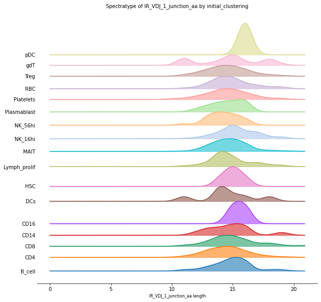
分别绘制各细胞簇的连接区长度分布，可以比较 CD4+、CD8+ 及 gdT-cell 等注释群体的峰值位置与分布宽度。解读时应同时核对受体链类型和细胞注释。

_ = ir.pl.spectratype(
    adata,
    cdr3_col="IR_VDJ_1_junction_aa",
    color="initial_clustering",
    viztype="curve",
    curve_layout="shifted",
    fig_kws={"figsize": [10, 10]},
    kde_kws={"kde_norm": False},
)

/home/juan.henao/.local/lib/python3.8/site-packages/scirpy/pl/base.py:262: UserWarning: FixedFormatter should only be used together with FixedLocator
  ax.set_yticklabels(order)

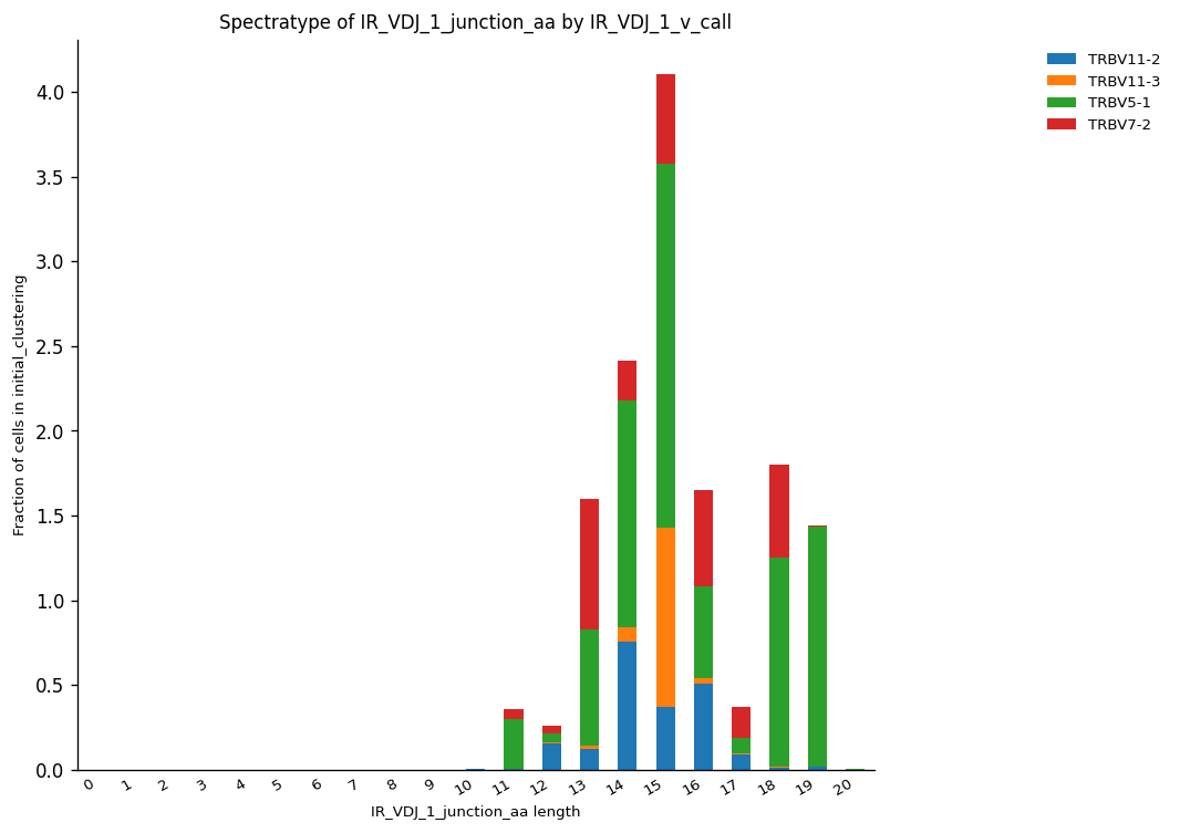
利用 AnnData 取子集，还能按 V 基因比较连接区长度。下面选择 TRBV5-1、TRBV11-2、TRBV7-2 和 TRBV11-3，这与上面的四基因列表不同。原教程结果中长度 15 较常见，TRBV5-1 和 TRBV11-3 较突出；此处长度仍指 junction_aa，而非 V 基因片段本身。代码还按 initial_clustering 指定归一化分组，解读纵轴时需考虑这一权重。

_ = ir.pl.spectratype(
    adata[
        adata.obs["IR_VDJ_1_v_call"].isin(
            ["TRBV5-1", "TRBV11-2", "TRBV7-2", "TRBV11-3"]
        ),
        :,
    ],
    cdr3_col="IR_VDJ_1_junction_aa",
    color="IR_VDJ_1_v_call",
    normalize="initial_clustering",
    fig_kws={"dpi": 120},
    figsize=[10, 10],
)

/home/juan.henao/.local/lib/python3.8/site-packages/anndata/compat/_overloaded_dict.py:106: ImplicitModificationWarning: Trying to modify attribute `._uns` of view, initializing view as actual.
  self.data[key] = value

序列基序分析¶

前面的分析概括了受体序列的整体属性。若要比较各氨基酸位置，可绘制序列标识图（sequence logo）：每个位置堆叠氨基酸字母，字母高度反映该位置的相对贡献，具体尺度取决于所用频率或信息量定义。

下面选择 V 基因为 TRBV5-1、TRBV11-2、TRBV7-2 或 TRBV11-3，且 VDJ 主链 junction_aa 长度为 15 的细胞，汇总其连接区序列绘图。代码实际使用四个 V 基因。

这里使用 Python 包 palmotif；它也用于 TCRdist3 等 TCR 分析工具。compute_motif 接收序列列表，svg_logo 将得到的标识图写入指定文件。

motif = compute_motif(
    adata[
        (
            adata.obs["IR_VDJ_1_v_call"].isin(
                ["TRBV5-1", "TRBV11-2", "TRBV7-2", "TRBV11-3"]
            )
        )
        & (adata.obs["IR_VDJ_1_junction_aa"].str.len() == 15),
        :,
    ]
    .obs["IR_VDJ_1_junction_aa"]
    .to_list()
)

_ = svg_logo(
    motif, "../_static/images/air_repertoire/logo_motif.svg", color_scheme="taylor"
)

图像保存为 logo_motif.svg，结果如下。

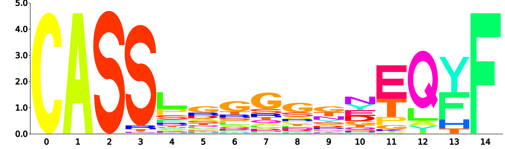
本例图中的主要模式是起始位置的 C-A-S 和末位的 F；第 14 位可见 Y、F、H、T，第四位则以 S 较突出，另有 R 和 T。这些模式可为后续序列研究或蛋白设计提供线索。由于输入按细胞汇总，扩增克隆会被重复计入；端部保守性还可来自 V/J 编码，不能直接解释为共同抗原特异性。

受体库比较¶

比较受体库可帮助识别样本间的相似性，研究不同条件下的免疫组成。默认 Jaccard 距离（Jaccard distance）使用克隆型是否出现的二值信息，而不是直接比较细胞丰度。Scirpy 可返回样本×克隆型的丰度矩阵（df）、样本间的 Jaccard 距离（dst）及层次聚类（hierarchical clustering）的连接矩阵（lk）。

df, dst, lk = ir.tl.repertoire_overlap(
    adata, "patient_id", target_col="cc_aa_identity", inplace=False
)

df

dst

array([1.        , 1.        , 1.        , 1.        , 1.        ,
       1.        , 1.        , 1.        , 1.        , 1.        ,
       1.        , 1.        , 1.        , 0.99982818, 1.        ])

lk

array([[3.        , 5.        , 0.99982818, 2.        ],
       [0.        , 1.        , 1.        , 2.        ],
       [2.        , 7.        , 1.        , 3.        ],
       [6.        , 8.        , 1.        , 5.        ],
       [4.        , 9.        , 1.        , 6.        ]])

可以用热图展示这些结果。原教程中，COVID-066 和 CV0902 的受体库相对接近，对应较小的 Jaccard 距离。两者来自不同中心：COVID-066 来自 Newcastle，CV0902 来自 Cambridge。

ir.pl.repertoire_overlap(
    adata, "patient_id", target_col="cc_aa_identity", heatmap_cats=["Centre"]
)

<seaborn.matrix.ClusterGrid at 0x7ff53cc2e2b0>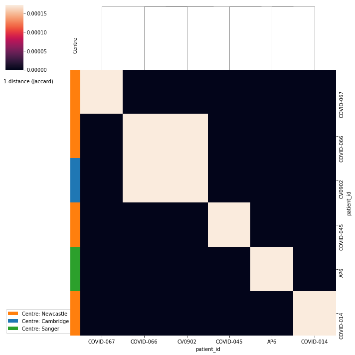

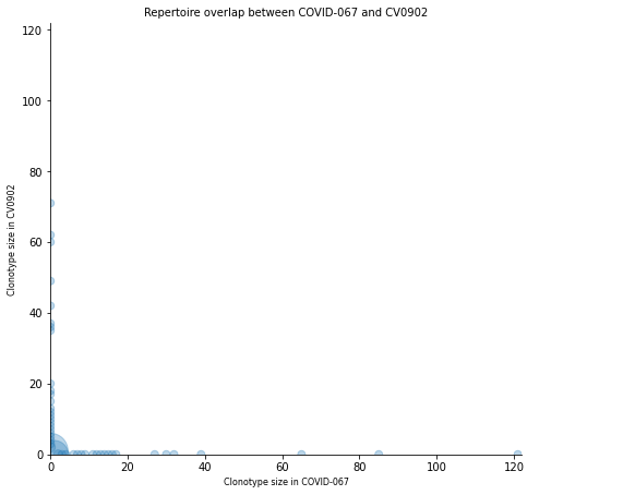
随后可比较一对样本中各克隆型的细胞数。散点图横、纵轴表示同一克隆型在两份样本中的丰度；具有相同坐标的克隆型还可汇总显示。下面实际比较的是 COVID-067 与 CV0902，并非上一段的 COVID-066。该绘图调用未显式指定 target_col，而前面使用 cc_aa_identity；运行时应核对默认键，确保采用同一克隆定义。

本例两个样本都包含大量小克隆。COVID-067 还包含少数细胞数较高的克隆；另一比较样本为 CV0902。

_ = ir.pl.repertoire_overlap(
    adata,
    "patient_id",
    pair_to_plot=["COVID-067", "CV0902"],
    fig_kws={"figsize": [10, 10]},
)

No handles with labels found to put in legend.

使用 Dandelion 分析 BCR 数据¶

以上演示了 TCR 库分析的常用步骤：定义克隆型、描述扩增与丰度、比较细胞类型和样本、分析 V(D)J 基因使用、连接区长度和序列基序。

这些思路也适用于 BCR 库分析 Gupta et al., 2015。不过，活化 B 细胞的免疫球蛋白可变区会积累突变，经选择后可提高抗原结合亲和力，这一过程称为 亲和力成熟（affinity maturation）。其中局部突变率显著高于一般背景的过程称为 体细胞高频突变（Somatic Hypermutation, SHM） Papavasiliou & Schatz, 2002。原文给出的约 10,000 倍是量级性的比较，并不表示每个受体经历固定倍数的突变；突变本身也不保证提高亲和力。因此，BCR 克隆识别通常需要容纳同一谱系内部的序列差异，可采用基于距离的方法。

这里使用 Dandelion 这一 Python 包。它可与 Scanpy 和 Scirpy 互操作，并提供基于序列距离的 BCR 克隆定义功能，下面介绍具体步骤 Stephenson et al., 2021。

import warnings

warnings.filterwarnings(
    "ignore",
    ".*IProgress not found*",
)
warnings.simplefilter(action="ignore", category=FutureWarning)

import dandelion as ddl
import matplotlib as mpl
import matplotlib.pyplot as plt
import pandas as pd
import scanpy as sc
import scirpy as ir
from palmotif import compute_motif, svg_logo

warnings.simplefilter(action="ignore", category=pd.errors.DtypeWarning)

sc.logging.print_versions()

WARNING: If you miss a compact list, please try `print_header`!
The `sinfo` package has changed name and is now called `session_info` to become more discoverable and self-explanatory. The `sinfo` PyPI package will be kept around to avoid breaking old installs and you can downgrade to 0.3.2 if you want to use it without seeing this message. For the latest features and bug fixes, please install `session_info` instead. The usage and defaults also changed slightly, so please review the latest README at https://gitlab.com/joelostblom/session_info.
-----
anndata     0.8.0
scanpy      1.8.2
sinfo       0.3.4
-----
Bio                         1.79
Levenshtein                 NA
PIL                         8.4.0
adjustText                  NA
airr                        1.4.1
anyio                       NA
asciitree                   NA
attr                        21.2.0
babel                       2.9.1
backcall                    0.2.0
beta_ufunc                  NA
binom_ufunc                 NA
brotli                      1.0.9
certifi                     2021.10.08
cffi                        1.15.0
changeo                     1.2.0
chardet                     4.0.0
charset_normalizer          2.0.8
cloudpickle                 2.0.0
colorama                    0.4.4
cycler                      0.10.0
cython_runtime              NA
dandelion                   0.2.4
dask                        2021.11.2
dateutil                    2.8.2
debugpy                     1.5.1
decorator                   5.1.0
defusedxml                  0.7.1
distance                    NA
entrypoints                 0.3
fasteners                   NA
fontTools                   4.28.2
fsspec                      0.7.4
google                      NA
h5py                        3.6.0
idna                        3.3
igraph                      0.9.8
importlib_resources         NA
ipykernel                   6.5.1
ipython_genutils            0.2.0
ipywidgets                  7.6.5
jedi                        0.18.1
jinja2                      3.0.3
joblib                      1.1.0
json5                       NA
jsonschema                  4.2.1
jupyter_server              1.12.1
jupyterlab_server           2.8.2
kiwisolver                  1.3.2
leidenalg                   0.8.8
llvmlite                    0.36.0
louvain                     0.7.0
lxml                        4.6.4
markupsafe                  2.0.1
matplotlib                  3.5.0
matplotlib_inline           NA
mizani                      0.7.4
mpl_toolkits                NA
natsort                     8.0.0
nbclassic                   NA
nbformat                    5.1.3
nbinom_ufunc                NA
networkx                    2.6.3
numba                       0.53.1
numcodecs                   0.9.1
numexpr                     2.7.3
numpy                       1.21.4
packaging                   21.3
palettable                  3.3.0
palmotif                    NA
pandas                      1.5.0
parasail                    1.3.3
parso                       0.8.2
patsy                       0.5.2
pexpect                     4.8.0
pickleshare                 0.7.5
pkg_resources               NA
plotnine                    0.9.0
polyleven                   NA
presto                      0.7.0
prometheus_client           NA
prompt_toolkit              3.0.23
ptyprocess                  0.7.0
pvectorc                    NA
pyarrow                     6.0.1
pydev_ipython               NA
pydevconsole                NA
pydevd                      2.6.0
pydevd_concurrency_analyser NA
pydevd_file_utils           NA
pydevd_plugins              NA
pydevd_tracing              NA
pygments                    2.10.0
pyparsing                   3.0.6
pyrsistent                  NA
pytoml                      NA
pytz                        2021.3
requests                    2.26.0
scipy                       1.7.3
scirpy                      0.11.1
seaborn                     0.11.2
send2trash                  NA
setuptools_scm              NA
six                         1.16.0
sklearn                     1.1.2
sniffio                     1.2.0
sparse                      0.13.0
statsmodels                 0.13.2
storemagic                  NA
svgwrite                    1.4.3
tables                      3.6.1
terminado                   0.12.1
texttable                   1.6.4
threadpoolctl               3.0.0
tlz                         0.11.2
toolz                       0.11.2
tornado                     6.1
tqdm                        4.62.3
tracerlib                   NA
traitlets                   5.1.1
typing_extensions           NA
urllib3                     1.26.7
wcwidth                     0.2.5
websocket                   1.2.1
yaml                        6.0
yamlordereddictloader       NA
zarr                        2.10.3
zipp                        NA
zmq                         22.3.0
-----
IPython             7.30.0
jupyter_client      7.1.0
jupyter_core        4.9.1
jupyterlab          3.2.4
notebook            6.4.6
-----
Python 3.8.12 (default, Nov 26 2021, 20:28:57) [GCC 10.2.1 20210110]
Linux-3.10.0-1160.25.1.el7.x86_64-x86_64-with-glibc2.29
48 logical CPU cores
-----
Session information updated at 2022-09-20 21:27

与 TCR 分析相同，先读取预处理得到的 .h5ad 文件。为缩短演示运行时间，这里选取 COVID-064 和 COVID-014 两名参与者的 BCR 数据用于比较。

path_data = "/home/icb/juan.henao/BestPracticeStart/data"

path_gex = f"{path_data}/BCR_filtered.h5ad"
adata_bcr = sc.read(path_gex)

adata = adata_bcr[adata_bcr.obs["patient_id"].isin(["COVID-064", "COVID-014"])].copy()

Dandelion 的数据互操作¶

Dandelion 使用自己的数据对象保存受体记录和细胞元数据，也提供与 AnnData/Scirpy 之间转换或传递结果的接口，以使用 Scanpy 等工具。

前面已将数据读入 AnnData，下面用 from_scirpy 转换为 Dandelion 对象。

vdjx = ddl.from_scirpy(adata)
vdjx

WARNING: Non-standard locus name ignored: Multi

Dandelion class object with n_obs = 6366 and n_contigs = 16953
    data: 'sequence_id', 'sequence', 'rev_comp', 'productive', 'v_call', 'd_call', 'j_call', 'sequence_alignment', 'germline_alignment', 'junction', 'junction_aa', 'v_cigar', 'd_cigar', 'j_cigar', 'c_call', 'consensus_count', 'duplicate_count', 'locus', 'cell_id', 'multi_chain', 'receptor_subtype', 'chain_pairing', 'receptor_type', 'is_cell', 'high_confidence', 'patient_id', 'rearrangement_status'
    metadata: 'locus_VDJ', 'locus_VJ', 'productive_VDJ', 'productive_VJ', 'v_call_VDJ', 'd_call_VDJ', 'j_call_VDJ', 'v_call_VJ', 'j_call_VJ', 'c_call_VDJ', 'c_call_VJ', 'junction_VDJ', 'junction_VJ', 'junction_aa_VDJ', 'junction_aa_VJ', 'v_call_B_VDJ', 'd_call_B_VDJ', 'j_call_B_VDJ', 'v_call_B_VJ', 'j_call_B_VJ', 'c_call_B_VDJ', 'c_call_B_VJ', 'productive_B_VDJ', 'productive_B_VJ', 'duplicate_count_B_VDJ', 'duplicate_count_B_VJ', 'isotype', 'isotype_status', 'locus_status', 'chain_status', 'rearrangement_status_VDJ', 'rearrangement_status_VJ'

克隆型定义¶

定义 BCR 克隆前，先删除 V、J 基因或 junction_aa 注释含 缺失值（NA data）的 contig 记录，再计算连接区长度；这不是删除“空细胞”。这里用 len(junction_aa) 得到氨基酸长度，但将结果写入 junction_length。后续使用核苷酸模型时应核对该字段的长度单位，不能将氨基酸长度与核苷酸长度混用。

vdjx.data["v_call"].replace("", np.nan, inplace=True)
vdjx.data.dropna(subset=["v_call"], inplace=True)

vdjx.data["j_call"].replace("", np.nan, inplace=True)
vdjx.data.dropna(subset=["j_call"], inplace=True)

vdjx.data["junction_aa"].replace("", np.nan, inplace=True)
vdjx.data.dropna(subset=["junction_aa"], inplace=True)

vdjx.data["junction_length"] = [len(a) for a in vdjx.data["junction_aa"]]

Dandelion 可使用考虑 SHM 替换倾向的距离模型识别 BCR 克隆，使有序列差异的受体仍可能归为同一克隆 Yaari et al., 2013 Cui et al., 2016。相关方法由 Immcantation 生态中的工具提供 Gupta et al., 2015 Vander Heiden et al., 2014。Dandelion 封装这些功能，减少在不同语言之间手动转换数据的工作，并可将结果用于 Scanpy 和 Scirpy。

五核苷酸（5-mer）上下文模型考虑一个位置及其上、下游各两个核苷酸，估计局部背景对突变倾向的影响 Yaari et al., 2013。相关模型使用同义突变（synonymous mutation）建立估计，即突变后密码子所编码的氨基酸不变，以减弱蛋白层面选择对估计的干扰 Yaari et al., 2013。

除 5-mer 模型外，也有不依赖邻近序列背景的单核苷酸替换模型。下表展示人和小鼠的单核苷酸替换代价；每一种碱基替换的代价固定，但不同替换并非都等价。注意：后面的代码实际使用 hh_s5f，即人类 5-mer 模型，不能把下表直接当成该模型的全部参数。

人类单核苷酸替换模型 Yaari et al., 2013：

核苷酸	A	C	G	T
A	0	1.21	0.64	1.16
C	1.21	0	1.16	0.64
G	0.64	1.16	0	1.21
T	1.16	0.64	1.21	0
N	0	0	0	0

小鼠单核苷酸替换模型 Cui et al., 2016：

核苷酸	A	C	G	T
A	0	1.51	0.32	1.17
C	1.51	0	1.17	0.32
G	0.32	1.17	0	1.51
T	1.17	0.32	1.51	0
N	0	0	0	0

基于距离定义克隆，需要选择阈值，将足够接近的受体序列归为候选克隆。Dandelion 封装了 Immcantation 的相关功能，通常先按 V/J 注释和连接区长度分组，再查看最近邻序列距离。距离分布有时呈双峰：较低距离可对应克隆内近缘序列，较高距离可对应无近缘匹配的序列 Gupta et al., 2015。可以在两部分之间选择阈值，但实际分布未必有清晰双峰，较高距离也不能一律解释为单细胞克隆。

ddl.pp.calculate_threshold(vdjx, model="hh_s5f", plot=False)
vdjx.threshold

/opt/python/lib/python3.8/site-packages/rpy2/robjects/pandas2ri.py:59: UserWarning: Error while trying to convert the column "productive". Fall back to string conversion. The error is: Series can only be of one type, or None (and here we have <class 'str'> and <class 'bool'>).
R[write to console]: Error in (function (db, sequenceColumn = "junction", vCallColumn = "v_call",  : 
  The locus column contains invalid loci annotations.

0.13319079238387194

选定距离模型和阈值后，再定义克隆。本例沿用原教程的 Dandelion 接口；较新版本的 define_clones 可能要求显式传入 dist，运行时应核对接口，并与前一步选出的阈值保持一致。

ddl.tl.define_clones(vdjx, key_added="changeo_clone_id", model="hh_s5f")

       START> DefineClones
        FILE> dandelion_define_clones_heavy-clone.tsv
   SEQ_FIELD> junction
     V_FIELD> v_call
     J_FIELD> j_call
 MAX_MISSING> 0
GROUP_FIELDS> None
      ACTION> set
        MODE> gene
    DISTANCE> 0.13319079238387194
     LINKAGE> single
       MODEL> hh_s5f
        NORM> len
         SYM> avg
       NPROC> 1

PROGRESS> [Grouping sequences] 21:28:26 (6828) 0.0 min

PROGRESS> [Assigning clones] 21:28:31 |####################| 100% (6,828) 0.1 min

 OUTPUT> dandelion_define_clones_heavy-clone.tsv
 CLONES> 4741
RECORDS> 6828
   PASS> 6828
   FAIL> 0
    END> DefineClones

定义克隆后需要计算网络布局。Dandelion 与 Scirpy 都能显示受体网络，但并非都依赖 igraph 布局。本例使用 sfdp；Dandelion 的相应实现使用 graph-tool 的 sfdp_layout，适合处理较大的网络，但不能据此断言它在所有数据上都比其他布局更省计算。

ddl.tl.generate_network(
    vdjx, key="sequence_alignment", layout_method="sfdp", clone_key="changeo_clone_id"
)

Setting up data: 14530it [00:01, 10889.53it/s]
Calculating distances... : 100%|██████████| 4720/4720 [00:02<00:00, 1758.62it/s]                                                                     
Generating edge list :   0%|          | 0/220 [00:00<?, ?it/s]                                                                                       /home/juan.henao/.local/lib/python3.8/site-packages/dandelion/tools/_network.py:259: SettingWithCopyWarning: 
A value is trying to be set on a copy of a slice from a DataFrame

See the caveats in the documentation: https://pandas.pydata.org/pandas-docs/stable/user_guide/indexing.html#returning-a-view-versus-a-copy
Generating edge list : 100%|██████████| 220/220 [00:00<00:00, 852.52it/s]                                                                            
Computing overlap : 100%|██████████| 4721/4721 [00:05<00:00, 846.28it/s]                                                                             
Linking edges : 100%|██████████| 4450/4450 [00:02<00:00, 1500.32it/s]

To benefit from faster layout computation, please install graph-tool: conda install -c conda-forge graph-tool

为了绘图，先将 Dandelion 的结果传入 AnnData，以使用 Scanpy 兼容的可视化接口。还可以用连线粗细表示受体序列距离：下面将边的距离 e 转换为 1/(e+1)，距离越小，线越粗；距离为零时线最粗。

ddl.tl.transfer(adata, vdjx, clone_key="changeo_clone_id", expanded_only=True)

edgeweights = [
    1 / (e + 1) for e in ddl.tl.extract_edge_weights(vdjx)
]  # invert and add 1 to each edge weight (e) so that distance of 0 becomes the thickest edge
# therefore, the thicker the line, the shorter the edit distance.

sc.set_figure_params(figsize=[10, 10])
_ = ddl.pl.clone_network(
    adata,
    color=["isotype_status"],
    legend_fontoutline=3,
    edges_width=edgeweights,
    size=50,
)

... storing 'changeo_clone_id' as categorical
... storing 'locus_VDJ' as categorical
... storing 'locus_VJ' as categorical
... storing 'productive_VDJ' as categorical
... storing 'productive_VJ' as categorical
... storing 'v_call_VDJ' as categorical
... storing 'd_call_VDJ' as categorical
... storing 'j_call_VDJ' as categorical
... storing 'v_call_VJ' as categorical
... storing 'j_call_VJ' as categorical
... storing 'c_call_VDJ' as categorical
... storing 'c_call_VJ' as categorical
... storing 'junction_VDJ' as categorical
... storing 'junction_VJ' as categorical
... storing 'junction_aa_VDJ' as categorical
... storing 'junction_aa_VJ' as categorical
... storing 'v_call_B_VDJ' as categorical
... storing 'd_call_B_VDJ' as categorical
... storing 'j_call_B_VDJ' as categorical
... storing 'v_call_B_VJ' as categorical
... storing 'j_call_B_VJ' as categorical
... storing 'c_call_B_VDJ' as categorical
... storing 'c_call_B_VJ' as categorical
... storing 'productive_B_VDJ' as categorical
... storing 'productive_B_VJ' as categorical
... storing 'isotype' as categorical
... storing 'isotype_status' as categorical
... storing 'locus_status' as categorical
... storing 'chain_status' as categorical
... storing 'rearrangement_status_VDJ' as categorical
... storing 'rearrangement_status_VJ' as categorical

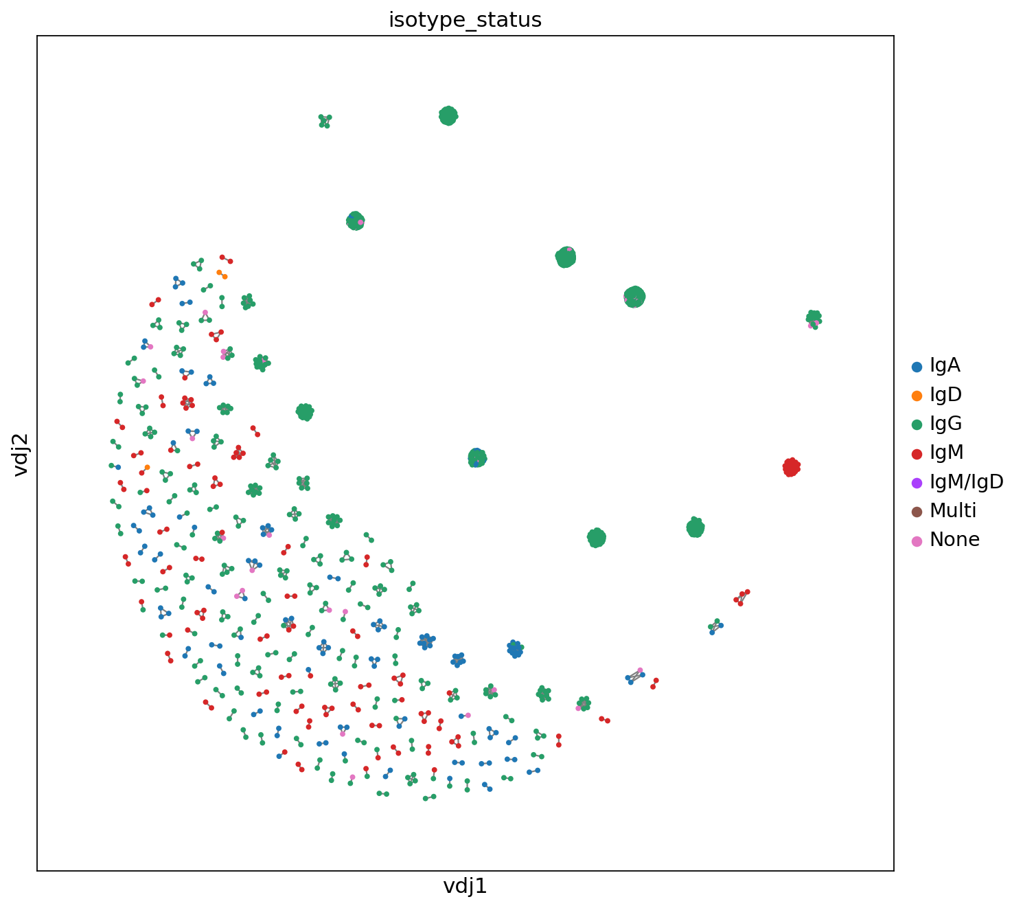
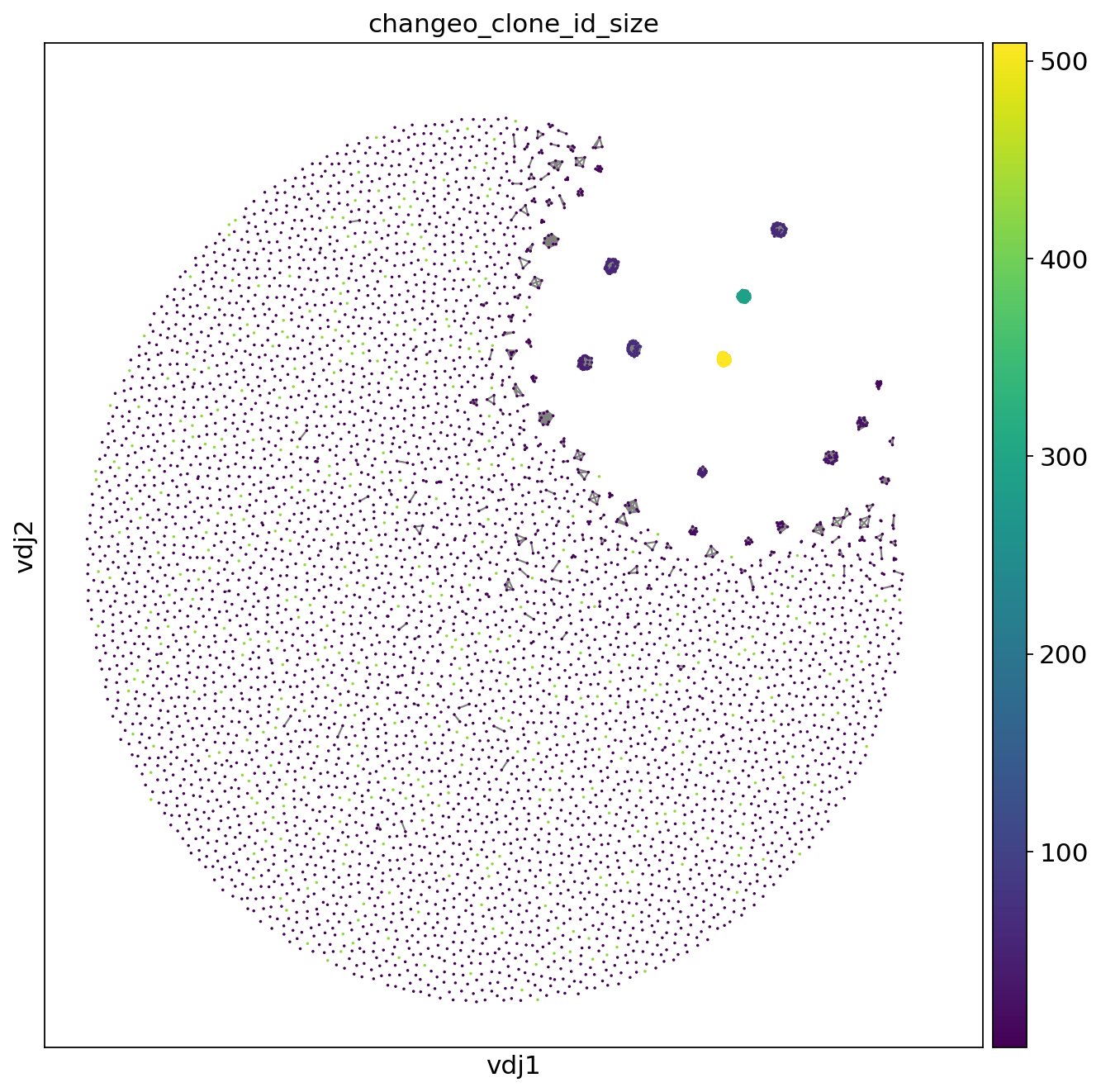
与前面的 Scirpy 图不同，此处 Dandelion 网络的点大小由绘图参数指定，不会自动表示克隆细胞数。先计算克隆大小，再把结果传入 AnnData 对象；下图用颜色表达克隆大小，所用的可视化接口兼容 Scanpy。

ddl.tl.clone_size(vdjx, clone_key="changeo_clone_id")
ddl.tl.transfer(adata, vdjx, clone_key="changeo_clone_id")

sc.set_figure_params(figsize=[10, 10])

_ = ddl.pl.clone_network(
    adata,
    color=["changeo_clone_id_size"],
    legend_loc="none",
    legend_fontoutline=3,
    edges_width=1,
    size=10,
)

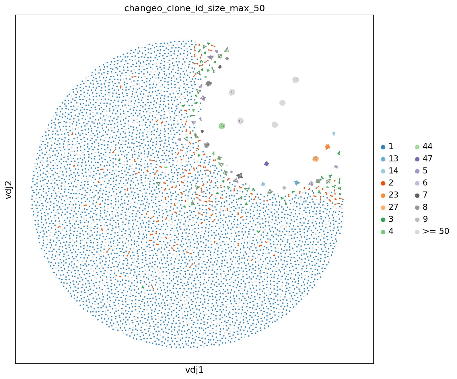
也可设置 max_size=50，将达到或超过 50 的克隆大小归为同一显示类别。这不会把克隆截取为 50 个细胞，也不会删除超出的细胞。

ddl.tl.clone_size(vdjx, clone_key="changeo_clone_id", max_size=50)
ddl.tl.transfer(adata, vdjx, clone_key="changeo_clone_id")

_ = ddl.pl.clone_network(
    adata,
    color=["changeo_clone_id_size_max_50"],
    ncols=2,
    legend_fontoutline=3,
    edges_width=1,
    palette="tab20c",
    size=20,
)

基因片段使用¶

与 TCR 分析一样，可以比较 BCR 的基因使用。Dandelion 提供按片段或链类别统计丰度的图形。

下面查看重链 V 基因的使用情况。min_clone_size=50 保留至少包含 50 个细胞的克隆，包含边界值 50。代码还显式排除 isotype_status 为 "Multi" 的多同型标记记录；这是一种减少歧义的分析选择，不能把这类细胞一律认定为无效受体。Dandelion 的链过滤行为还取决于所用函数、版本与参数，应与这里的元数据过滤分开理解。

mpl.rcParams.update(mpl.rcParamsDefault)
_ = ddl.pl.barplot(
    vdjx[vdjx.metadata.isotype_status != "Multi"],
    clone_key="changeo_clone_id",
    color="v_call_VDJ",
    min_clone_size=50,
    figsize=[15, 8],
)

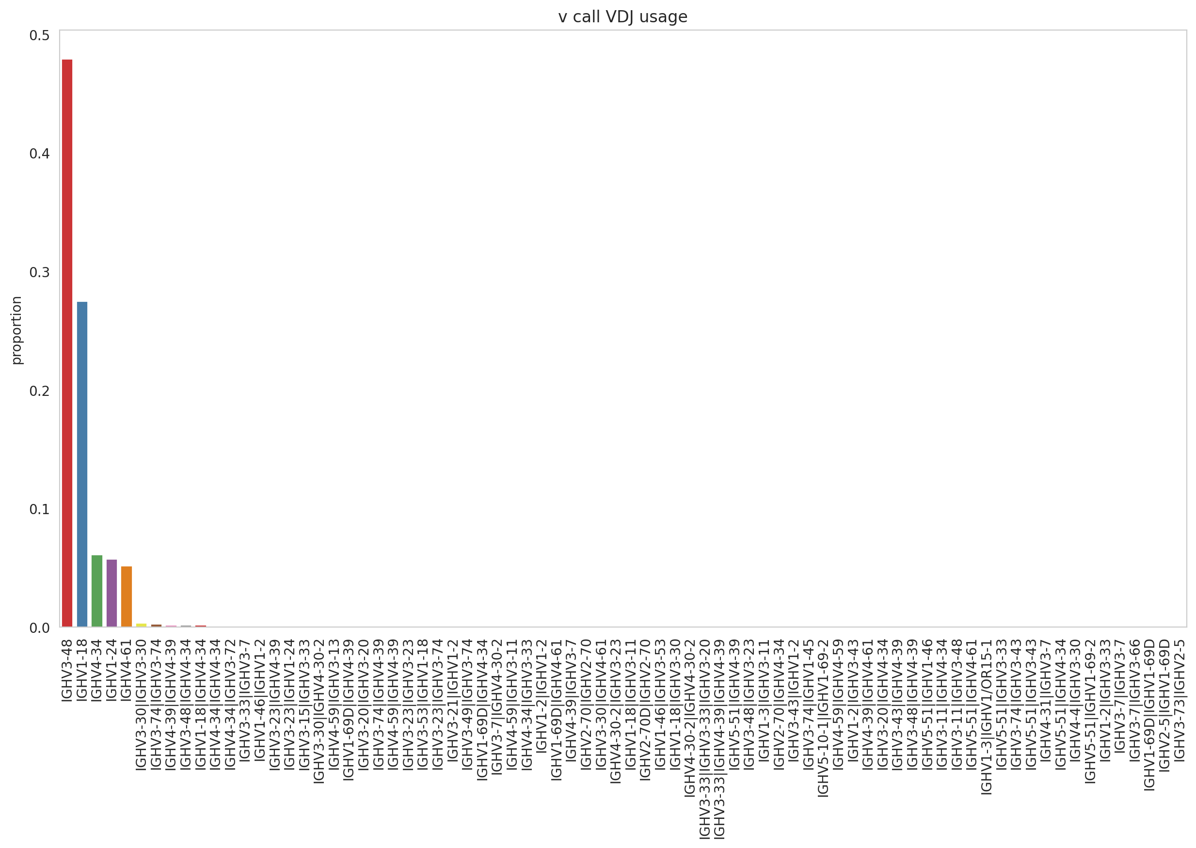
在本例选出的较大克隆中，IGHV3-48 和 IGHV1-18 对应细胞较多。这说明所选数据中的 V 基因使用不均匀，但优势扩增克隆本身就可能驱动这一结果，不能单独证明重组偏好。

加入免疫球蛋白同型（immunoglobulin isotype）信息后，可以进一步比较这些 V 基因在不同同型中的分布。

_ = (
    ddl.pl.stackedbarplot(
        vdjx[vdjx.metadata.isotype_status != "Multi"],
        clone_key="changeo_clone_id",
        color="v_call_VDJ",
        groupby="isotype_status",
        min_clone_size=50,
        xtick_rotation=90,
        figsize=(18, 8),
        normalize=True,
    ),
)

_ = plt.legend(bbox_to_anchor=(1, 1), loc="upper left", frameon=False)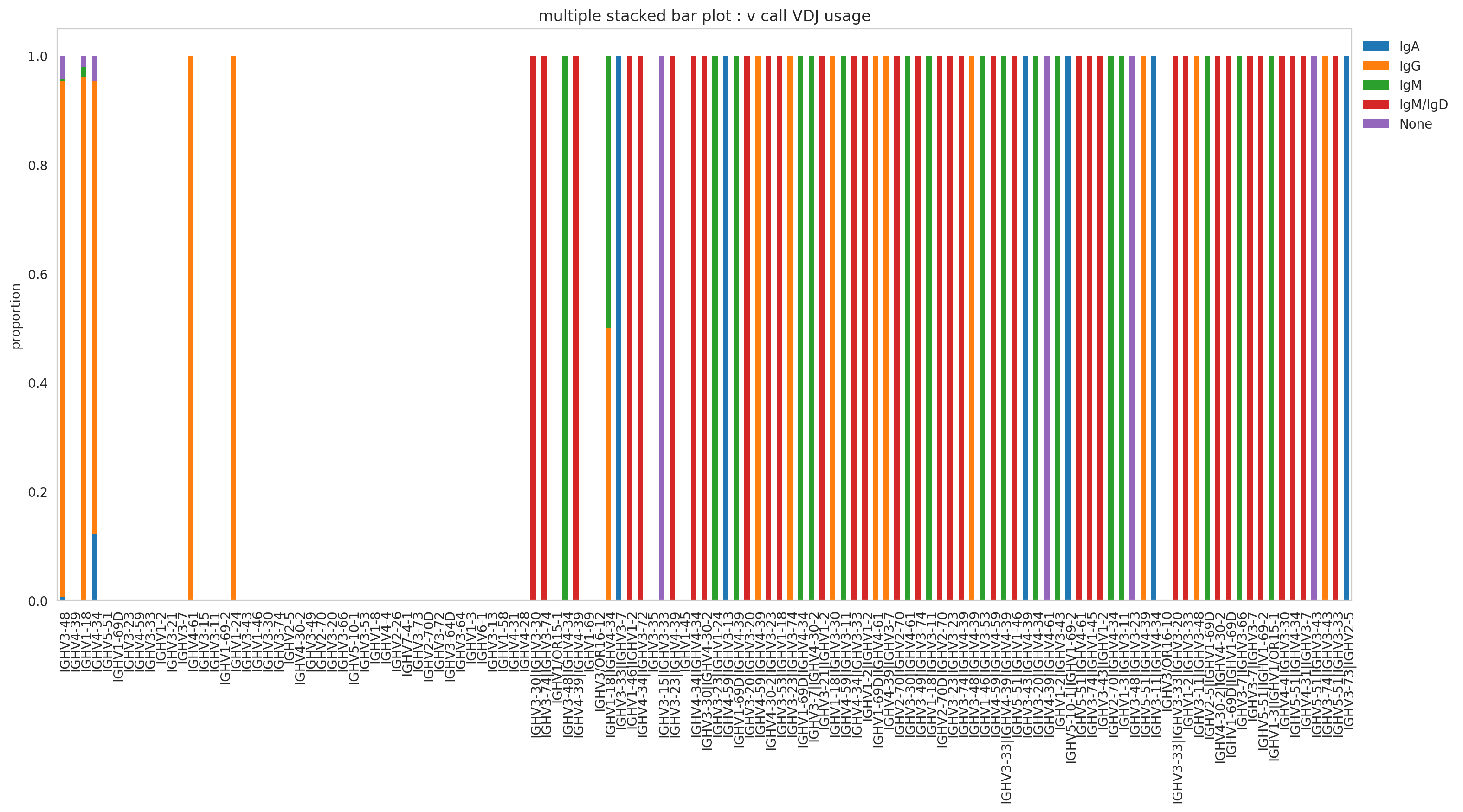

原教程图中，与 IGHV3-48 和 IGHV1-18 相关的较大克隆主要呈免疫球蛋白 G（immunoglobulin G, IgG）同型。由于扩增的 IgG 细胞较多，其他同型的使用模式可能在汇总图中不明显。

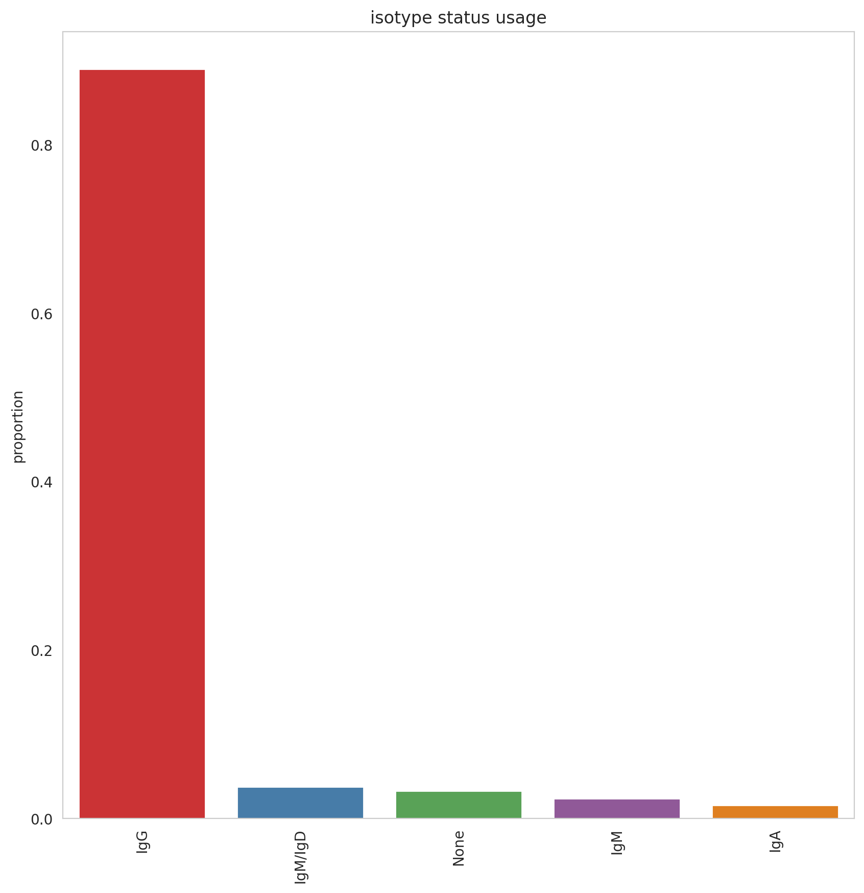
下面按同型汇总至少 50 个细胞的克隆。原教程中，这些大克隆几乎都由 IgG 细胞构成，说明所选数据的扩增组成；仅凭 IgG 占比并不能确定具体抗原或免疫应答的诱因。

_ = ddl.pl.barplot(
    vdjx[vdjx.metadata.isotype_status != "Multi"],
    clone_key="changeo_clone_id",
    color="isotype_status",
    min_clone_size=50,
    figsize=[10, 10],
)

谱型¶

确定较大克隆及其同型后，继续比较连接区长度。下面排除 isotype_status="Multi" 的记录，并显式要求 changeo_clone_id_size > 50；这里是严格大于 50，与前面 min_clone_size=50 包含边界的条件略有不同。

本例 BCR 重链的连接区长度分布有两个突出峰值：23 个氨基酸最多，其次为 15 个氨基酸。这里的 junction_length 来自前面计算的氨基酸序列长度。

_ = ddl.pl.spectratype(
    vdjx[
        (vdjx.metadata.isotype_status != "Multi")
        & (vdjx.metadata.changeo_clone_id_size > 50.0)
    ],
    color="junction_length",
    groupby="v_call",
    locus="IGH",
    figsize=(10, 10),
)
_ = plt.legend(bbox_to_anchor=(1, 1), loc="upper left", frameon=False)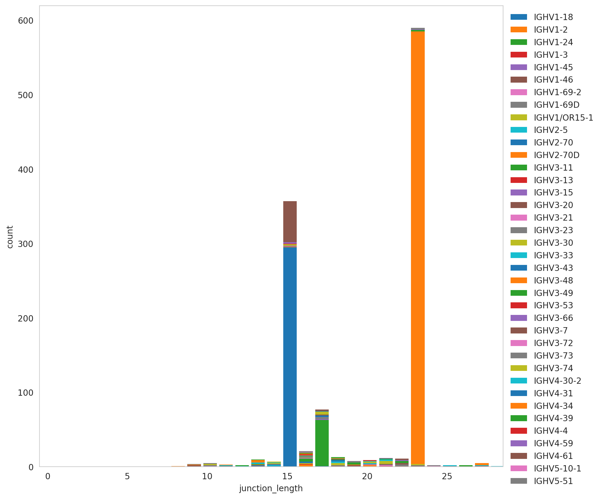

序列基序分析¶

根据谱型结果，可进一步选择与 IGHV3-48 和 IGHV1-18 这两个 V 基因之一对应的受体，分别比较长度为 15 和 23 个氨基酸的重链连接区。分析对象是 junction_aa，不是 V 基因片段本身；先查看长度为 15 的序列。

ddl.tl.transfer(adata, vdjx, clone_key="changeo_clone_id")

motif = compute_motif(
    adata[
        (adata.obs["IR_VDJ_1_v_call"].isin(["IGHV3-48", "IGHV1-18"]))
        & (adata.obs["junction_aa_VDJ"].str.len() == 15),
        :,
    ]
    .obs["junction_aa_VDJ"]
    .to_list()
)

_ = svg_logo(
    motif, "../_static/images/air_repertoire/bcr_logo_motif.svg", color_scheme="taylor"
)

本例长度为 15 的连接区中，多数位置由少数氨基酸主导，部分位置则较多样。这个图按细胞汇总，未再次应用前面的克隆大小和 Multi 筛选；扩增克隆及 V/J 编码的保守位置都可能影响模式，不能直接将其解释为抗原特异基序。

随后对使用同样两个 V 基因、但重链 junction_aa 长度为 23 个氨基酸的细胞绘图，以比较连接区模式。

motif = compute_motif(
    adata[
        (adata.obs["IR_VDJ_1_v_call"].isin(["IGHV3-48", "IGHV1-18"]))
        & (adata.obs["junction_aa_VDJ"].str.len() == 23),
        :,
    ]
    .obs["junction_aa_VDJ"]
    .to_list()
)

_ = svg_logo(
    motif, "../_static/images/air_repertoire/bcr2_logo_motif.svg", color_scheme="taylor"
)

References¶

Polonsky, M., Chain, B., & Friedman, N. (2016). Clonal expansion under the microscope: studying lymphocyte activation and differentiation using live-cell imaging. Immunology and Cell Biology, 94(3), 242–249.
Naxerova, K. (2020). Clonal competition in a confined space. Nature Genetics, 52(6), 553–554.
Ashcroft, P., Manz, M. G., & Bonhoeffer, S. (2017). Clonal dominance and transplantation dynamics in hematopoietic stem cell compartments. PLoS Computational Biology, 13(10), e1005803.
Kim, T.-S., & Shin, E.-C. (2019). The activation of bystander CD8+ T cells and their roles in viral infection. Experimental & Molecular Medicine, 51(12), 1–9.
Travlos, I. S., Cheimona, N., Roussis, I., & Bilalis, D. J. (2018). Weed-species abundance and diversity indices in relation to tillage systems and fertilization. Frontiers in Environmental Science, 6, 11.
Elhanati, Y., Murugan, A., Callan Jr, C. G., Mora, T., & Walczak, A. M. (2014). Quantifying selection in immune receptor repertoires. Proceedings of the National Academy of Sciences, 111(27), 9875–9880.
Chernyshev, M., Kaduk, M., Corcoran, M., & Hedestam, G. B. K. (2021). VDJ Gene Usage in IgM Repertoires of Rhesus and Cynomolgus Macaques. Frontiers in Immunology, 12.
Ciupe, S. M., Devlin, B. H., Markert, M. L., & Kepler, T. B. (2013). Quantification of total T-cell receptor diversity by flow cytometry and spectratyping. BMC Immunology, 14(1), 1–12.
Gupta, N. T., Vander Heiden, J. A., Uduman, M., Gadala-Maria, D., Yaari, G., & Kleinstein, S. H. (2015). Change-O: a toolkit for analyzing large-scale B cell immunoglobulin repertoire sequencing data. Bioinformatics, 31(20), 3356–3358.
Papavasiliou, F. N., & Schatz, D. G. (2002). Somatic hypermutation of immunoglobulin genes: merging mechanisms for genetic diversity. Cell, 109(2), S35–S44.
Stephenson, E., Reynolds, G., Botting, R. A., Calero-Nieto, F. J., Morgan, M. D., Tuong, Z. K., Bach, K., Sungnak, W., Worlock, K. B., Yoshida, M., & others. (2021). Single-cell multi-omics analysis of the immune response in COVID-19. Nature Medicine, 27(5), 904–916.
Yaari, G., Vander Heiden, J. A., Uduman, M., Gadala-Maria, D., Gupta, N., Stern, J. N., O’Connor, K. C., Hafler, D. A., Laserson, U., Vigneault, F., & others. (2013). Models of somatic hypermutation targeting and substitution based on synonymous mutations from high-throughput immunoglobulin sequencing data. Frontiers in Immunology, 4, 358.
Cui, A., Di Niro, R., Vander Heiden, J. A., Briggs, A. W., Adams, K., Gilbert, T., O’Connor, K. C., Vigneault, F., Shlomchik, M. J., & Kleinstein, S. H. (2016). A model of somatic hypermutation targeting in mice based on high-throughput Ig sequencing data. The Journal of Immunology, 197(9), 3566–3574.
Vander Heiden, J. A., Yaari, G., Uduman, M., Stern, J. N., O’Connor, K. C., Hafler, D. A., Vigneault, F., & Kleinstein, S. H. (2014). pRESTO: a toolkit for processing high-throughput sequencing raw reads of lymphocyte receptor repertoires. Bioinformatics, 30(13), 1930–1932.